Computing time-of-flight for WFM data

Wavelength-frame-multiplication (WFM) is a technique commonly used at long-pulse facilities to improve the resolution of the results measured at the neutron detectors. See for example the article by Schmakat et al. (2020) for a description of how WFM works.

In this notebook, we show how to use Scippneutron’s tof module to find the boundaries of the WFM frames, and apply a time correction to each frame, in order to obtain more accurate a time-of-flight coordinate, from which a wavelength can be computed.

import numpy as np
import plopp as pp
import scipp as sc
import sciline as sl
from scippneutron.chopper import DiskChopper
from scippneutron.tof import unwrap
from scippneutron.tof import chopper_cascade

Setting up the beamline

Creating the beamline choppers

We begin by defining the chopper settings for our beamline. In principle, the chopper setting could simply be read from a NeXus file.

For this example, we create choppers modeled on the V20 ESS beamline at HZB. It consists of 5 choppers:

• 2 WFM choppers

• 2 frame-overlap choppers

• 1 pulse-overlap chopper

The first 4 choppers have 6 openings (also known as cutouts), while the last one only has a single opening.

wfm1 = DiskChopper(
    frequency=sc.scalar(-70.0, unit="Hz"),
    beam_position=sc.scalar(0.0, unit="deg"),
    phase=sc.scalar(-47.10, unit="deg"),
    axle_position=sc.vector(value=[0, 0, 6.6], unit="m"),
    slit_begin=sc.array(
        dims=["cutout"],
        values=np.array([83.71, 140.49, 193.26, 242.32, 287.91, 330.3]) + 15.0,
        unit="deg",
    ),
    slit_end=sc.array(
        dims=["cutout"],
        values=np.array([94.7, 155.79, 212.56, 265.33, 314.37, 360.0]) + 15.0,
        unit="deg",
    ),
    slit_height=sc.scalar(10.0, unit="cm"),
    radius=sc.scalar(30.0, unit="cm"),
)

wfm2 = DiskChopper(
    frequency=sc.scalar(-70.0, unit="Hz"),
    beam_position=sc.scalar(0.0, unit="deg"),
    phase=sc.scalar(-76.76, unit="deg"),
    axle_position=sc.vector(value=[0, 0, 7.1], unit="m"),
    slit_begin=sc.array(
        dims=["cutout"],
        values=np.array([65.04, 126.1, 182.88, 235.67, 284.73, 330.32]) + 15.0,
        unit="deg",
    ),
    slit_end=sc.array(
        dims=["cutout"],
        values=np.array([76.03, 141.4, 202.18, 254.97, 307.74, 360.0]) + 15.0,
        unit="deg",
    ),
    slit_height=sc.scalar(10.0, unit="cm"),
    radius=sc.scalar(30.0, unit="cm"),
)

foc1 = DiskChopper(
    frequency=sc.scalar(-56.0, unit="Hz"),
    beam_position=sc.scalar(0.0, unit="deg"),
    phase=sc.scalar(-62.40, unit="deg"),
    axle_position=sc.vector(value=[0, 0, 8.8], unit="m"),
    slit_begin=sc.array(
        dims=["cutout"],
        values=np.array([74.6, 139.6, 194.3, 245.3, 294.8, 347.2]),
        unit="deg",
    ),
    slit_end=sc.array(
        dims=["cutout"],
        values=np.array([95.2, 162.8, 216.1, 263.1, 310.5, 371.6]),
        unit="deg",
    ),
    slit_height=sc.scalar(10.0, unit="cm"),
    radius=sc.scalar(30.0, unit="cm"),
)

foc2 = DiskChopper(
    frequency=sc.scalar(-28.0, unit="Hz"),
    beam_position=sc.scalar(0.0, unit="deg"),
    phase=sc.scalar(-12.27, unit="deg"),
    axle_position=sc.vector(value=[0, 0, 15.9], unit="m"),
    slit_begin=sc.array(
        dims=["cutout"],
        values=np.array([98.0, 154.0, 206.8, 255.0, 299.0, 344.65]),
        unit="deg",
    ),
    slit_end=sc.array(
        dims=["cutout"],
        values=np.array([134.6, 190.06, 237.01, 280.88, 323.56, 373.76]),
        unit="deg",
    ),
    slit_height=sc.scalar(10.0, unit="cm"),
    radius=sc.scalar(30.0, unit="cm"),
)

pol = DiskChopper(
    frequency=sc.scalar(-14.0, unit="Hz"),
    beam_position=sc.scalar(0.0, unit="deg"),
    phase=sc.scalar(0.0, unit="deg"),
    axle_position=sc.vector(value=[0, 0, 17.0], unit="m"),
    slit_begin=sc.array(
        dims=["cutout"],
        values=np.array([40.0]),
        unit="deg",
    ),
    slit_end=sc.array(
        dims=["cutout"],
        values=np.array([240.0]),
        unit="deg",
    ),
    slit_height=sc.scalar(10.0, unit="cm"),
    radius=sc.scalar(30.0, unit="cm"),
)

disk_choppers = {"wfm1": wfm1, "wfm2": wfm2, "foc1": foc1, "foc2": foc2, "pol": pol}

It is possible to visualize the properties of the choppers by inspecting their repr:

wfm1

DiskChopper

(cutout: 6)

• axle_position

  scipp

  Variable

  ()

  vector3

  m

  [0. 0. 6.6]
• frequency

  scipp

  Variable

  ()

  float64

  Hz

  -70.0
• beam_position

  scipp

  Variable

  ()

  float64

  deg

  0.0
• phase

  scipp

  Variable

  ()

  float64

  deg

  -47.1
• slit_begin

  scipp

  Variable

  (cutout: 6)

  float64

  deg

  98.71, 155.490, ..., 302.910, 345.3
• slit_end

  scipp

  Variable

  (cutout: 6)

  float64

  deg

  109.7, 170.790, ..., 329.370, 375.0
• slit_height

  scipp

  Variable

  (cutout: 6)

  float64

  cm

  10.0, 10.0, ..., 10.0, 10.0
• radius

  scipp

  Variable

  ()

  float64

  cm

  30.0

Adding a detector

We also have a detector, which we place 26 meters away from the source.

Ltotal = sc.scalar(26.0, unit="m")

Convert the choppers

Lastly, we convert our disk choppers to a simpler chopper representation used by the chopper_cascade module.

choppers = {
    key: chopper_cascade.Chopper.from_disk_chopper(
        chop, pulse_frequency=sc.scalar(14.0, unit="Hz"), npulses=1
    )
    for key, chop in disk_choppers.items()
}

Creating some neutron events

We create a semi-realistic set of neutron events based on the ESS pulse.

from scippneutron.tof.fakes import FakeBeamlineEss

ess_beamline = FakeBeamlineEss(
    choppers=choppers,
    monitors={"detector": Ltotal},
    run_length=sc.scalar(1 / 14, unit="s") * 14,
    events_per_pulse=200_000,
)

The initial birth times and wavelengths of the generated neutrons can be visualized (for a single pulse):

one_pulse = ess_beamline.source.data["pulse", 0]
one_pulse.hist(time=300).plot() + one_pulse.hist(wavelength=300).plot()

From this fake beamline, we extract the raw neutron signal at our detector:

raw_data = ess_beamline.get_monitor("detector")

# Visualize
raw_data.hist(event_time_offset=300).sum("pulse").plot()

The total number of neutrons in our sample data that make it through the to detector is:

raw_data.sum().value

203715.0

Using the chopper cascade to chop the pulse

The chopper_cascade module can now be used to chop a pulse of neutrons using the choppers created above.

Create a pulse of neutrons

We then create a (fake) pulse of neutrons, whose time and wavelength ranges cover our ESS pulse above:

time_min = sc.scalar(0.0, unit='ms')
time_max = sc.scalar(3.4, unit='ms')
wavs_min = sc.scalar(0.01, unit='angstrom')
wavs_max = sc.scalar(10.0, unit='angstrom')

frames = chopper_cascade.FrameSequence.from_source_pulse(
    time_min=time_min,
    time_max=time_max,
    wavelength_min=wavs_min,
    wavelength_max=wavs_max,
)

Propagate the neutrons through the choppers

We are now able to propagate the pulse of neutrons through the chopper cascade, chopping away the parts of the pulse that do not make it through.

For this, we need to decide how far we want to propagate the neutrons, by choosing a distance to our detector. We set this to 32 meters here.

# Chop the frames
frames = frames.chop(choppers.values())

# Propagate the neutrons to the detector
at_sample = frames.propagate_to(Ltotal)

# Visualize the results
cascade_fig, cascade_ax = at_sample.draw()

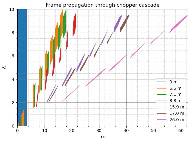
We can now see that at the detector (pink color), we have 6 sub-pulses of neutrons, where the longest wavelength of one frame is very close to the shortest wavelength of the next frame.

Computing the time-of-flight coordinate using Sciline

Setting up the workflow

We will now construct a workflow to compute the time-of-flight coordinate from the neutron events above, taking into account the choppers in the beamline.

workflow = sl.Pipeline(
    unwrap.unwrap_providers()
    + unwrap.time_of_flight_providers()
    + unwrap.time_of_flight_origin_from_choppers_providers(wfm=True)
)

workflow[unwrap.PulsePeriod] = sc.reciprocal(ess_beamline.source.frequency)
workflow[unwrap.PulseStride | None] = None
workflow[unwrap.SourceTimeRange] = time_min, time_max
workflow[unwrap.SourceWavelengthRange] = wavs_min, wavs_max
workflow[unwrap.Choppers] = choppers

workflow[unwrap.Ltotal] = Ltotal
workflow[unwrap.RawData] = raw_data

workflow.visualize(unwrap.TofData)

Checking the frame bounds

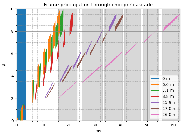
We can check that the bounds for the frames the workflow computes agrees with the chopper-cascade diagram

bounds = workflow.compute(unwrap.FrameAtDetector).subbounds()
bounds

scipp.DataGroup

(subframe: 6, bound: 2)

• time

  scipp

  Variable

  (subframe: 6, bound: 2)

  float64

  s

  0.016, 0.023, ..., 0.056, 0.063
• wavelength

  scipp

  Variable

  (subframe: 6, bound: 2)

  float64

  Å

  2.007, 3.514, ..., 7.964, 9.528

for b in sc.collapse(bounds["time"], keep="bound").values():
    cascade_ax.axvspan(
        b[0].to(unit="ms").value,
        b[1].to(unit="ms").value,
        color="gray",
        alpha=0.3,
        zorder=-5,
    )

cascade_fig

There should be one vertical band matching the extent of each pink polygon, which there is.

Computing a time-of-flight coordinate

We will now use our workflow to obtain our event data with a time-of-flight coordinate:

tofs = workflow.compute(unwrap.TofData)
tofs

scipp.DataArray (12.63 MB)

• Dimensions:
  • pulse: 14
• Coordinates: (1)
  • Ltotal
    ()
    float64
    m
    19.4

    Values:
    array(19.4)

• Data: (1)
  • (pulse)
    DataArrayView
    binned data [len=14396, len=14450, ..., len=14797, len=14571]

    dim='event',
    content=DataArray(
              dims=(event: 203715),
              data=float64[counts],
              coords={'id':int64, 'toa':float64[µs], 'event_time_offset':float64[s],
                      'time_offset':float64[s], 'pulse_time':datetime64[µs],
                      'tof':float64[s], 'time_zero':datetime64[µs]},
              masks={'blocked_by_others':bool})

Histogramming the data for a plot should show a profile with 6 bumps that correspond to the frames:

edges = sc.linspace("tof", 0.005, 0.05, 300, unit="s")
tofs.bins.concat().hist(tof=edges).plot()

Converting to wavelength

We can now convert our new time-of-flight coordinate to a neutron wavelength, using tranform_coords:

from scippneutron.conversion.graph.beamline import beamline
from scippneutron.conversion.graph.tof import elastic

# Perform coordinate transformation
graph = {**beamline(scatter=False), **elastic("tof")}
wav_wfm = tofs.transform_coords("wavelength", graph=graph)

# Define wavelength bin edges
wavs = sc.linspace("wavelength", 2, 10, 301, unit="angstrom")

wav_wfm.hist(wavelength=wavs).sum("pulse").plot()

Comparing to the ground truth

As a consistency check, because we actually know the wavelengths of the neutrons we created, we can compare the true neutron wavelengths to those we computed above.

ground_truth = ess_beamline.model_result["detector"].data.flatten(to="event")
ground_truth = ground_truth[~ground_truth.masks["blocked_by_others"]]

pp.plot(
    {
        "wfm": wav_wfm.hist(wavelength=wavs).sum("pulse"),
        "ground_truth": ground_truth.hist(wavelength=wavs),
    }
)