two_theta gravity correction

The impact of gravity matters in some instruments where large wavelengths are used. This includes SANS and reflectometry. In those cases, we need to take gravity into account when computing the scattering angle \(2\theta\). This document derives the expression that ScippNeutron uses in this case. Further, this expression contains an approximation that is explained and analyzed further down.

Derivation and approximation

After scattering, the neutron travels along curve

\[\begin{split}C: \vec{c}(t) = \begin{pmatrix}v_x t \\ -\frac{g}{2}t^2 + v_y t \\ v_z t\end{pmatrix}.\end{split}\]

with initial velocity

\[\begin{split}\vec{v} = v \begin{pmatrix}\cos(\phi)\sin(2\theta) \\ \sin(\phi)\sin(2\theta) \\ \cos(2\theta)\end{pmatrix}, \quad v = \frac{h}{m_n \lambda}.\end{split}\]

For a detector located at \(z_d = v_z t_d\), this means that the neutron is detected at

\[\begin{split}\vec{p} = \begin{pmatrix}x_d \\ y_d \\ z_d\end{pmatrix} = \begin{pmatrix}v_x t_d \\ -\frac{g}{2}t_d^2 + v_y t_d \\ v_z t_d\end{pmatrix}.\end{split}\]

To determine the scattering angles, we can consider the point where the neutron would be detected without gravity:

\[\begin{split}\vec{p}' = \begin{pmatrix}x_d \\ y'_d \\ z_d\end{pmatrix} = \begin{pmatrix}v_x t_d \\ v_y t_d \\ v_z t_d\end{pmatrix} = v t_d \begin{pmatrix}\cos(\phi)\sin(2\theta) \\ \sin(\phi)\sin(2\theta) \\ \cos(2\theta)\end{pmatrix}\end{split}\]

Thus

\[\tan(2\theta) = \frac{\sqrt{x_d^2 + y_d^{\prime\,2}}}{z_d}, \quad y_d' = y_d + \frac{g}{2} t_d^2 = y_d + \frac{g m_n^2 \lambda^2}{2 h^2} L_2^{\prime\,2}\]

with

\[L'_2 = \frac{z_d}{\cos(2\theta)}\]

Solving these equations for \(2 \theta\) is difficult. However, the impact of gravity is small, so we approximate \(L_2 \approx L'_2\). And \(L_2 = |\vec{p}|\) is readily available from pixel positions. Note that Mantid uses the same approximation, see Q1D.

Validity of the approximation

We found evidence that the approximation has an unexpectedly large impact on the end result (\(I(Q)\)). Initially, this was observed by using \(\sin(2 \theta) = \sqrt{x^2 + y'^2} / L_2\) instead of the tangent-based equation for \(2 \theta\). This equation is also an approximation. But it would be exact if it used \(L'_2\) in the denominator instead of \(L_2\).

With SANS2D data, we found a relative difference of \(~10^{-5}\) in the resulting \(2 \theta\). This amounted to a relative difference of \(~10^{-4}\) in \(I(Q)\) which is within statistical uncertainties. However, LOKI is rather long and allows for measuring relatively large angles. So it is a priori not clear that the approximation holds.

To test it, we

1. Pick a set of values of \(\lambda\), \(z_d\), \(2 \theta\), \(\phi\).

2. Compute \(\vec{p}\) from those.

3. Compute \(2 \theta\) using \(\vec{p}\) and the equation for \(\tan(2\theta)\).

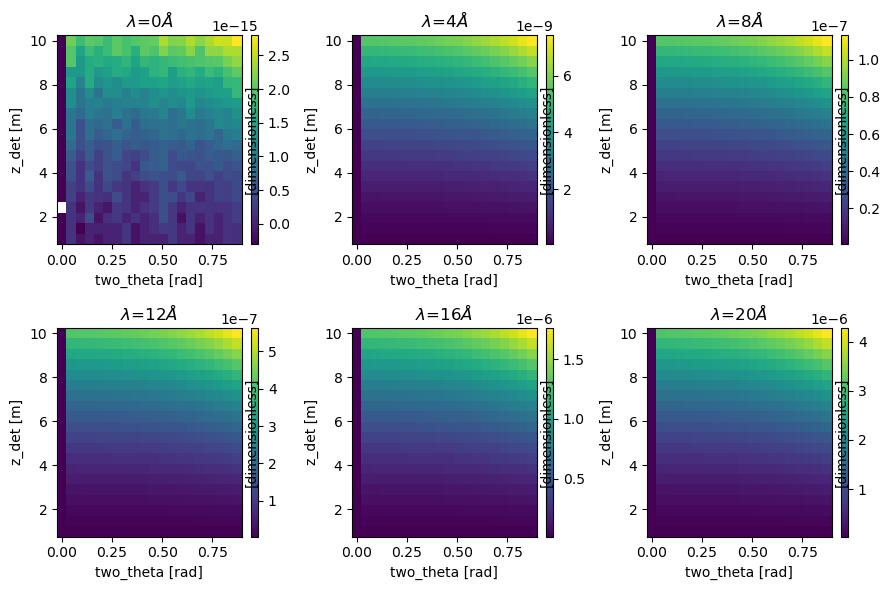
The code below outputs a figure that shows the relative difference true_two_theta -approx_two_theta) / true_two_theta for \(\phi = 90^{\circ}\). true_two_theta is the input value for \(2 \theta\) and approx_two_theta is the result of the computation described above. Parameters were chosen in realistic ranges for LOKI. The error of the approximation is no larger than \(~10^{-6}\). So the impact on the final \(I(Q)\) will likely be within statistical uncertainties and can be neglected.

import matplotlib.pyplot as plt
import scipp as sc
import scipp.constants


def two_theta_approx(
    *,
    wavelength,
    two_theta,
    phi,
    z_det,
):
    v = sc.constants.h / sc.constants.m_n / wavelength
    v_x = v * sc.cos(phi) * sc.sin(two_theta)
    v_y = v * sc.sin(phi) * sc.sin(two_theta)

    t_det = z_det / (v * sc.cos(two_theta))
    x_det = v_x * t_det
    y_det = v_y * t_det
    y_det = y_det - (sc.constants.g * t_det**2 / 2).to(unit=y_det.unit)

    L2 = sc.sqrt(x_det**2 + y_det**2 + z_det**2)
    drop = (
        sc.constants.g
        / 2
        * sc.constants.m_n**2
        * wavelength**2
        / sc.constants.h**2
        * L2**2
    )
    y_det_prime = y_det + drop.to(unit=y_det.unit)

    return sc.atan2(y=sc.sqrt(x_det**2 + y_det_prime**2), x=z_det)


wavelength = sc.linspace("wavelength", 0.1, 20.0, 6, unit="Å")
two_theta = sc.linspace("two_theta", 0.0, 50.0, 20, unit="deg").to(unit="rad")
phi = sc.scalar(90.0, unit="deg").to(unit="rad")
z_det = sc.linspace("z_det", 1.0, 10.0, 20, unit="m")

approx = two_theta_approx(
    wavelength=wavelength, two_theta=two_theta, phi=phi, z_det=z_det
)
error = (two_theta - approx) / two_theta
error = sc.DataArray(
    error,
    coords={"two_theta": two_theta, "z_det": z_det, "phi": phi, "wavelength": wavelength},
)

fig, axs = plt.subplots(2, 3, figsize=(9, 6))
for i, ax in zip(range(error.sizes["wavelength"]), axs.flat, strict=True):
    da = error["wavelength", i]
    da.plot(ax=ax, title=f"$\\lambda$={da.coords['wavelength'].value:.0f}$\\AA$")
fig.tight_layout()