Chopper Cascades#
Overview#
The chopper_cascade module provides utilities for computing time and wavelength bounds of a neutron pulse (or sub-pulses) propagating through a chopper cascade. This is useful for designing chopper systems, as well as predicting the data recorded when using techniques such as wavelength-frame multiplication (WFM).
It is currently under development and not fully functional.
Example: WFM chopper cascade#
As an example, consider the WFM chopper cascade from the tof package documentation.
[1]:
from scippneutron.tof import chopper_cascade
import scipp as sc
import matplotlib as mpl

mpl.rcParams['figure.dpi'] = 300
Defining choppers#
Choppers are defined by their position along the beam path, and the opening and closing times of their cutouts.
[2]:
params = {'wfm1': {'open': [-0.000396, 0.001286, 0.005786, 0.008039, 0.010133, 0.012080, 0.013889, 0.015571],
                   'close': [0.000654, 0.002464, 0.006222, 0.008646, 0.010899, 0.012993, 0.014939, 0.016750],
                   'distance': 6.6},
          'wfm2': {'open': [0.000654, 0.002451, 0.006222, 0.008645, 0.010898, 0.012993, 0.014940, 0.016737],
                   'close': [0.001567, 0.003641, 0.006658, 0.009252, 0.011664, 0.013759, 0.015853, 0.017927],
                   'distance': 7.1},
          'foc1': {'open': [-0.000139, 0.002460, 0.006796, 0.010020, 0.012733, 0.015263, 0.017718, 0.020317],
                   'close': [0.000640, 0.003671, 0.007817, 0.011171, 0.013814, 0.016146, 0.018497, 0.021528],
                   'distance': 8.8},
          'foc2': {'open': [-0.000306, 0.010939, 0.016495, 0.021733, 0.026416, 0.030880, 0.035409],
                   'close': [0.002582, 0.014570, 0.020072, 0.024730, 0.029082, 0.033316, 0.038297],
                   'distance': 15.9}
         }

choppers = sc.DataGroup(
    {name: chopper_cascade.Chopper(
        distance=sc.scalar(param['distance'], unit='m'),
        time_open=sc.array(dims=('cutout',), values=param['open'], unit='s'),
        time_close=sc.array(dims=('cutout',), values=param['close'], unit='s')
    ) for name, param in params.items()}
)
We can now initialize a frame-sequence and apply the chopper cascade to it:
[3]:
frames = chopper_cascade.FrameSequence.from_source_pulse(
    time_min=sc.scalar(0.0, unit='ms'),
    time_max=sc.scalar(4.0, unit='ms'),  # ESS pulse is 3 ms, but it has a tail
    wavelength_min=sc.scalar(0.0, unit='angstrom'),
    wavelength_max=sc.scalar(10.0, unit='angstrom'),
)
frames = frames.chop(choppers.values())
at_sample = frames.propagate_to(sc.scalar(26.0, unit='m'))

at_sample.draw()
[3]:
(<Figure size 1920x1440 with 1 Axes>,
 <Axes: title={'center': 'Frame propagation through chopper cascade'}, xlabel='ms', ylabel='Å'>)
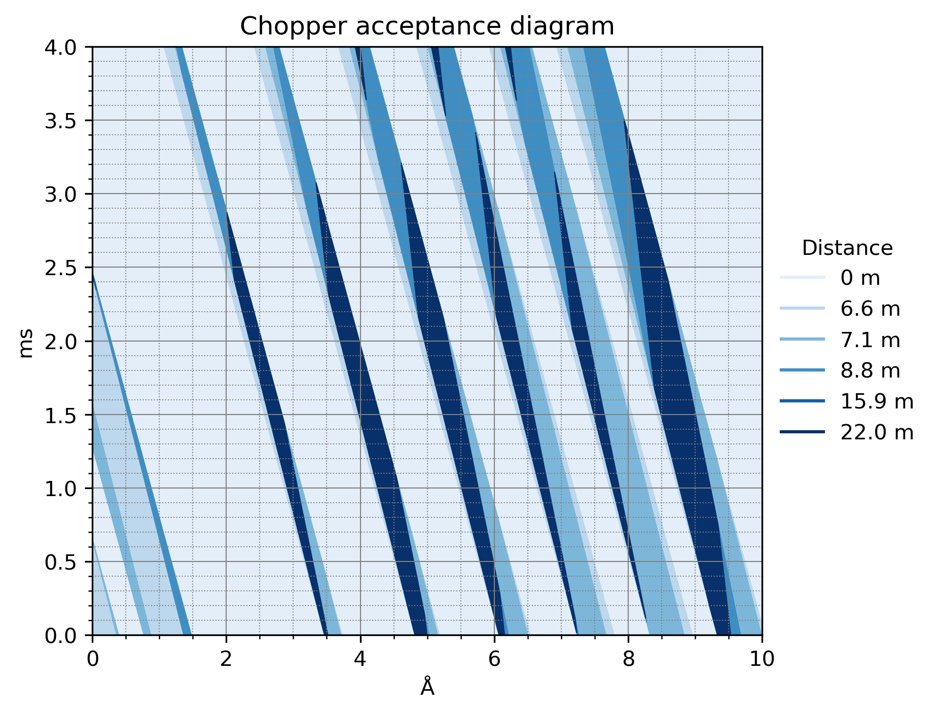
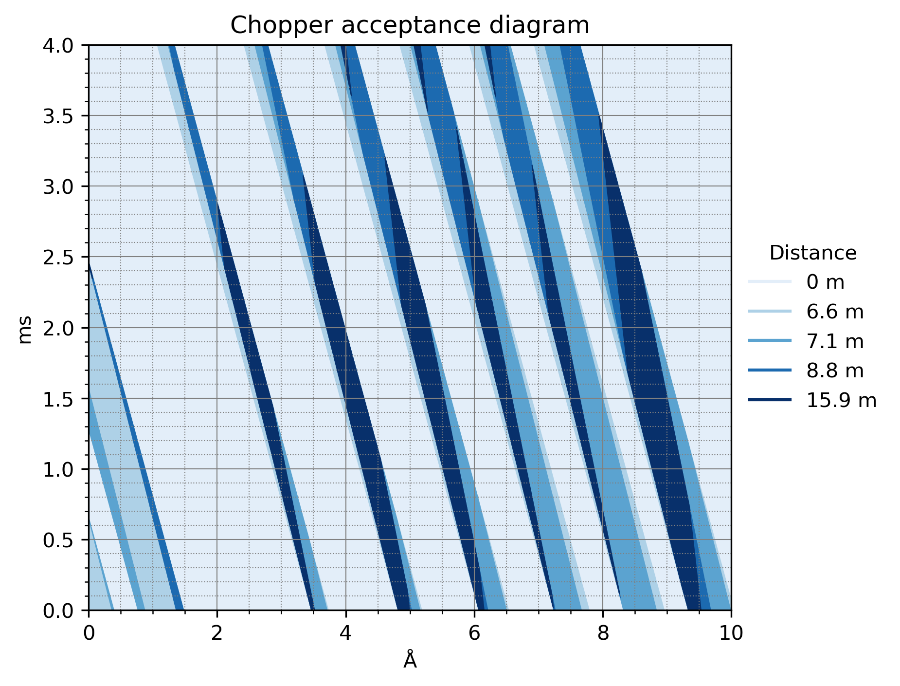
We can also draw a chopper acceptance diagram, which is essentially the same as above, but propagated back to the source pulse distance:
[4]:
frames.acceptance_diagram()
[4]:
(<Figure size 1920x1440 with 1 Axes>,
 <Axes: title={'center': 'Chopper acceptance diagram'}, xlabel='Å', ylabel='ms'>)
Frame unwrapping#
For unwrapping frames, we need the bounds of the entire frame, to determine times at which to cut. Since \(L_2\) can be different for every detector, this cutting time is different for every detector. We can compute the frame bounds at a common distance, e.g., the sample, and propagate the bounds to the detectors:
[5]:
bounds = at_sample[-1].bounds()
chopper_cascade.propagate_times(
    time=bounds['time'],
    wavelength=bounds['wavelength'],
    distance=sc.linspace('L2', 1.0, 2.0, 100, unit='m'),
)
[5]:
- (L2: 100, bound: 2)float64s0.002, 0.065, ..., 0.002, 0.067
Values:
array([[0.00246   , 0.06503264],
       [0.00246   , 0.06505697],
       [0.00246   , 0.0650813 ],
       [0.00246   , 0.06510563],
       [0.00246   , 0.06512996],
       [0.00246   , 0.06515429],
       [0.00246   , 0.06517862],
       [0.00246   , 0.06520295],
       [0.00246   , 0.06522728],
       [0.00246   , 0.06525161],
       [0.00246   , 0.06527594],
       [0.00246   , 0.06530027],
       [0.00246   , 0.0653246 ],
       [0.00246   , 0.06534892],
       [0.00246   , 0.06537325],
       [0.00246   , 0.06539758],
       [0.00246   , 0.06542191],
       [0.00246   , 0.06544624],
       [0.00246   , 0.06547057],
       [0.00246   , 0.0654949 ],
       [0.00246   , 0.06551923],
       [0.00246   , 0.06554356],
       [0.00246   , 0.06556789],
       [0.00246   , 0.06559222],
       [0.00246   , 0.06561655],
       [0.00246   , 0.06564088],
       [0.00246   , 0.06566521],
       [0.00246   , 0.06568954],
       [0.00246   , 0.06571387],
       [0.00246   , 0.0657382 ],
       [0.00246   , 0.06576253],
       [0.00246   , 0.06578685],
       [0.00246   , 0.06581118],
       [0.00246   , 0.06583551],
       [0.00246   , 0.06585984],
       [0.00246   , 0.06588417],
       [0.00246   , 0.0659085 ],
       [0.00246   , 0.06593283],
       [0.00246   , 0.06595716],
       [0.00246   , 0.06598149],
       [0.00246   , 0.06600582],
       [0.00246   , 0.06603015],
       [0.00246   , 0.06605448],
       [0.00246   , 0.06607881],
       [0.00246   , 0.06610314],
       [0.00246   , 0.06612747],
       [0.00246   , 0.0661518 ],
       [0.00246   , 0.06617613],
       [0.00246   , 0.06620046],
       [0.00246   , 0.06622478],
       [0.00246   , 0.06624911],
       [0.00246   , 0.06627344],
       [0.00246   , 0.06629777],
       [0.00246   , 0.0663221 ],
       [0.00246   , 0.06634643],
       [0.00246   , 0.06637076],
       [0.00246   , 0.06639509],
       [0.00246   , 0.06641942],
       [0.00246   , 0.06644375],
       [0.00246   , 0.06646808],
       [0.00246   , 0.06649241],
       [0.00246   , 0.06651674],
       [0.00246   , 0.06654107],
       [0.00246   , 0.0665654 ],
       [0.00246   , 0.06658973],
       [0.00246   , 0.06661406],
       [0.00246   , 0.06663839],
       [0.00246   , 0.06666272],
       [0.00246   , 0.06668704],
       [0.00246   , 0.06671137],
       [0.00246   , 0.0667357 ],
       [0.00246   , 0.06676003],
       [0.00246   , 0.06678436],
       [0.00246   , 0.06680869],
       [0.00246   , 0.06683302],
       [0.00246   , 0.06685735],
       [0.00246   , 0.06688168],
       [0.00246   , 0.06690601],
       [0.00246   , 0.06693034],
       [0.00246   , 0.06695467],
       [0.00246   , 0.066979  ],
       [0.00246   , 0.06700333],
       [0.00246   , 0.06702766],
       [0.00246   , 0.06705199],
       [0.00246   , 0.06707632],
       [0.00246   , 0.06710065],
       [0.00246   , 0.06712497],
       [0.00246   , 0.0671493 ],
       [0.00246   , 0.06717363],
       [0.00246   , 0.06719796],
       [0.00246   , 0.06722229],
       [0.00246   , 0.06724662],
       [0.00246   , 0.06727095],
       [0.00246   , 0.06729528],
       [0.00246   , 0.06731961],
       [0.00246   , 0.06734394],
       [0.00246   , 0.06736827],
       [0.00246   , 0.0673926 ],
       [0.00246   , 0.06741693],
       [0.00246   , 0.06744126]])
For WFM, we need to compute subframe time cutting points. Again, \(L_2\) can be different for every detector, so we need to compute the cutting points for every detector:
[6]:
bounds = at_sample[-1].subbounds()
bounds
[6]:
- timescippVariable(subframe: 10, bound: 2)float64s0.002, 0.003, ..., 0.056, 0.063
- wavelengthscippVariable(subframe: 10, bound: 2)float64Å0.0, 0.059, ..., 7.937, 9.529
[7]:
chopper_cascade.propagate_times(
    time=bounds['time'],
    wavelength=bounds['wavelength'],
    distance=sc.linspace('L2', 1.0, 2.0, 100, unit='m'),
)
[7]:
- (L2: 100, subframe: 10, bound: 2)float64s0.002, 0.003, ..., 0.060, 0.067
Values:
array([[[0.00246   , 0.00274724],
        [0.01656897, 0.02398398],
        [0.02586316, 0.03408453],
        ...,
        [0.04608932, 0.04684825],
        [0.05023934, 0.05649482],
        [0.05767942, 0.06503264]],

       [[0.00246   , 0.00274739],
        [0.01657409, 0.02399295],
        [0.02587169, 0.03409728],
        ...,
        [0.04610506, 0.04686442],
        [0.05025696, 0.05651591],
        [0.05769969, 0.06505697]],

       [[0.00246   , 0.00274754],
        [0.01657921, 0.02400192],
        [0.02588021, 0.03411003],
        ...,
        [0.04612081, 0.04688059],
        [0.05027457, 0.056537  ],
        [0.05771995, 0.0650813 ]],

       ...,

       [[0.00246   , 0.00276182],
        [0.01706593, 0.02485433],
        [0.02669009, 0.03532142],
        ...,
        [0.04761669, 0.04841648],
        [0.05194819, 0.05854081],
        [0.05964523, 0.0673926 ]],

       [[0.00246   , 0.00276197],
        [0.01707105, 0.0248633 ],
        [0.02669861, 0.03533417],
        ...,
        [0.04763244, 0.04843265],
        [0.05196581, 0.05856191],
        [0.0596655 , 0.06741693]],

       [[0.00246   , 0.00276213],
        [0.01707617, 0.02487227],
        [0.02670714, 0.03534692],
        ...,
        [0.04764818, 0.04844882],
        [0.05198342, 0.058583  ],
        [0.05968576, 0.06744126]]])
Note that subframes may in principle overlap, and this may depend on the detector. We therefore call subframe_bounds at a common location and propagate the result, otherwise we would get a different number of subframes for different detectors.