DREAM in WFM mode

In this notebook, we show how to use Scippneutron’s tof module to find the boundaries of the WFM frames for the DREAM instrument. We then apply a time correction to each frame to compute a time-of-flight coordinate, from which a wavelength can be derived.

import plopp as pp
import scipp as sc
import sciline as sl
from scippneutron.chopper import DiskChopper
from scippneutron.tof import unwrap
from scippneutron.tof import chopper_cascade

Setting up the beamline

Creating the beamline choppers

We begin by defining the chopper settings for our beamline. In principle, the chopper setting could simply be read from a NeXus file.

The DREAM instrument has

• 2 pulse-shaping choppers (PSC)

• 1 overlap chopper (OC)

• 1 band-control chopper (BCC)

• 1 T0 chopper

psc1 = DiskChopper(
    frequency=sc.scalar(14.0, unit="Hz"),
    beam_position=sc.scalar(0.0, unit="deg"),
    phase=sc.scalar(286 - 180, unit="deg"),
    axle_position=sc.vector(value=[0, 0, 6.145], unit="m"),
    slit_begin=sc.array(
        dims=["cutout"],
        values=[-1.23, 70.49, 84.765, 113.565, 170.29, 271.635, 286.035, 301.17],
        unit="deg",
    ),
    slit_end=sc.array(
        dims=["cutout"],
        values=[1.23, 73.51, 88.035, 116.835, 175.31, 275.565, 289.965, 303.63],
        unit="deg",
    ),
    slit_height=sc.scalar(10.0, unit="cm"),
    radius=sc.scalar(30.0, unit="cm"),
)

psc2 = DiskChopper(
    frequency=sc.scalar(-14.0, unit="Hz"),
    beam_position=sc.scalar(0.0, unit="deg"),
    phase=sc.scalar(-236, unit="deg"),
    axle_position=sc.vector(value=[0, 0, 6.155], unit="m"),
    slit_begin=sc.array(
        dims=["cutout"],
        values=[-1.23, 27.0, 55.8, 142.385, 156.765, 214.115, 257.23, 315.49],
        unit="deg",
    ),
    slit_end=sc.array(
        dims=["cutout"],
        values=[1.23, 30.6, 59.4, 145.615, 160.035, 217.885, 261.17, 318.11],
        unit="deg",
    ),
    slit_height=sc.scalar(10.0, unit="cm"),
    radius=sc.scalar(30.0, unit="cm"),
)

oc = DiskChopper(
    frequency=sc.scalar(14.0, unit="Hz"),
    beam_position=sc.scalar(0.0, unit="deg"),
    phase=sc.scalar(297 - 180 - 90, unit="deg"),
    axle_position=sc.vector(value=[0, 0, 6.174], unit="m"),
    slit_begin=sc.array(dims=["cutout"], values=[-27.6 * 0.5], unit="deg"),
    slit_end=sc.array(dims=["cutout"], values=[27.6 * 0.5], unit="deg"),
    slit_height=sc.scalar(10.0, unit="cm"),
    radius=sc.scalar(30.0, unit="cm"),
)

bcc = DiskChopper(
    frequency=sc.scalar(112.0, unit="Hz"),
    beam_position=sc.scalar(0.0, unit="deg"),
    phase=sc.scalar(240 - 180, unit="deg"),
    axle_position=sc.vector(value=[0, 0, 9.78], unit="m"),
    slit_begin=sc.array(dims=["cutout"], values=[-36.875, 143.125], unit="deg"),
    slit_end=sc.array(dims=["cutout"], values=[36.875, 216.875], unit="deg"),
    slit_height=sc.scalar(10.0, unit="cm"),
    radius=sc.scalar(30.0, unit="cm"),
)

t0 = DiskChopper(
    frequency=sc.scalar(28.0, unit="Hz"),
    beam_position=sc.scalar(0.0, unit="deg"),
    phase=sc.scalar(280 - 180, unit="deg"),
    axle_position=sc.vector(value=[0, 0, 13.05], unit="m"),
    slit_begin=sc.array(dims=["cutout"], values=[-314.9 * 0.5], unit="deg"),
    slit_end=sc.array(dims=["cutout"], values=[314.9 * 0.5], unit="deg"),
    slit_height=sc.scalar(10.0, unit="cm"),
    radius=sc.scalar(30.0, unit="cm"),
)

disk_choppers = {"psc1": psc1, "psc2": psc2, "oc": oc, "bcc": bcc, "t0": t0}

It is possible to visualize the properties of the choppers by inspecting their repr:

psc2

DiskChopper

(cutout: 8)

• axle_position

  scipp

  Variable

  ()

  vector3

  m

  [0. 0. 6.155]
• frequency

  scipp

  Variable

  ()

  float64

  Hz

  -14.0
• beam_position

  scipp

  Variable

  ()

  float64

  deg

  0.0
• phase

  scipp

  Variable

  ()

  int64

  deg

  -236
• slit_begin

  scipp

  Variable

  (cutout: 8)

  float64

  deg

  -1.23, 27.0, ..., 257.230, 315.490
• slit_end

  scipp

  Variable

  (cutout: 8)

  float64

  deg

  1.23, 30.6, ..., 261.170, 318.110
• slit_height

  scipp

  Variable

  (cutout: 8)

  float64

  cm

  10.0, 10.0, ..., 10.0, 10.0
• radius

  scipp

  Variable

  ()

  float64

  cm

  30.0

Adding a detector

Ltotal = sc.scalar(76.55 + 1.125, unit="m")

Convert the choppers

Lastly, we convert our disk choppers to a simpler chopper representation used by the chopper_cascade module.

choppers = {
    key: chopper_cascade.Chopper.from_disk_chopper(
        chop,
        pulse_frequency=sc.scalar(14.0, unit="Hz"),
        npulses=1,
    )
    for key, chop in disk_choppers.items()
}

Creating some neutron events

We create a semi-realistic set of neutron events based on the ESS pulse.

from scippneutron.tof.fakes import FakeBeamlineEss

ess_beamline = FakeBeamlineEss(
    choppers=choppers,
    monitors={"detector": Ltotal},
    run_length=sc.scalar(1 / 14, unit="s") * 4,
    events_per_pulse=200_000,
)

The initial birth times and wavelengths of the generated neutrons can be visualized (for a single pulse):

one_pulse = ess_beamline.source.data["pulse", 0]
one_pulse.hist(time=300).plot() + one_pulse.hist(wavelength=300).plot()

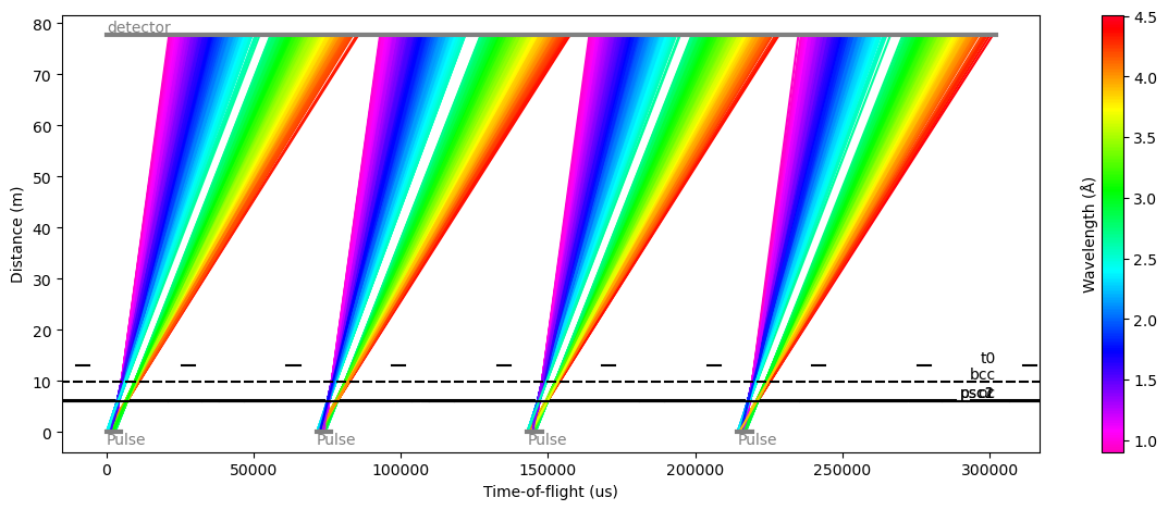
ess_beamline.model_result.plot()

Plot(ax=<Axes: xlabel='Time-of-flight (us)', ylabel='Distance (m)'>, fig=<Figure size 1200x480 with 2 Axes>)

From this fake beamline, we extract the raw neutron signal at our detector:

raw_data = ess_beamline.get_monitor("detector")

# Visualize
raw_data.hist(event_time_offset=300).sum("pulse").plot()

The total number of neutrons in our sample data that make it through the to detector is:

raw_data.sum().value

72459.0

Using the chopper cascade to chop the pulse

The chopper_cascade module can now be used to chop a pulse of neutrons using the choppers created above.

Create a pulse of neutrons

We then create a (fake) pulse of neutrons, whose time and wavelength ranges are close to that of our ESS pulse above:

pulse_tmin = one_pulse.coords["time"].min()
pulse_tmax = one_pulse.coords["time"].max()
pulse_wmin = one_pulse.coords["wavelength"].min()
pulse_wmax = one_pulse.coords["wavelength"].max()

frames = chopper_cascade.FrameSequence.from_source_pulse(
    time_min=pulse_tmin,
    time_max=pulse_tmax,
    wavelength_min=pulse_wmin,
    wavelength_max=pulse_wmax,
)

Propagate the neutrons through the choppers

We are now able to propagate the pulse of neutrons through the chopper cascade, chopping away the parts of the pulse that do not make it through.

For this, we need to decide how far we want to propagate the neutrons, by choosing a distance to our detector. We set this to 32 meters here.

# Chop the frames
chopped = frames.chop(choppers.values())

# Propagate the neutrons to the detector
at_sample = chopped.propagate_to(Ltotal)

# Visualize the results
cascade_fig, cascade_ax = at_sample.draw()

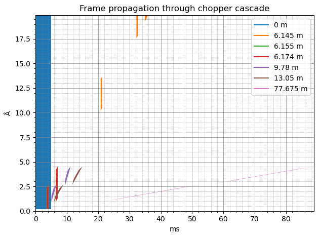
We can now see that at the detector (pink color), we have 2 sub-pulses of neutrons, where the longest wavelength of one frame is very close to the shortest wavelength of the next frame.

Computing the time-of-flight coordinate using Sciline

Setting up the workflow

We will now construct a workflow to compute the time-of-flight coordinate from the neutron events above, taking into account the choppers in the beamline.

workflow = sl.Pipeline(
    unwrap.unwrap_providers()
    + unwrap.time_of_flight_providers()
    + unwrap.time_of_flight_origin_from_choppers_providers(wfm=True)
)

workflow[unwrap.PulsePeriod] = sc.reciprocal(ess_beamline.source.frequency)
workflow[unwrap.PulseStride | None] = None
workflow[unwrap.SourceTimeRange] = pulse_tmin, pulse_tmax
workflow[unwrap.SourceWavelengthRange] = pulse_wmin, pulse_wmax
workflow[unwrap.Choppers] = choppers

workflow[unwrap.Ltotal] = Ltotal
workflow[unwrap.RawData] = raw_data

workflow.visualize(unwrap.TofData)

Checking the frame bounds

We can check that the bounds for the frames the workflow computes agrees with the chopper-cascade diagram

bounds = workflow.compute(unwrap.CleanFrameAtDetector).subbounds()
bounds

scipp.DataGroup

(subframe: 2, bound: 2)

• time

  scipp

  Variable

  (subframe: 2, bound: 2)

  float64

  s

  0.055, 0.089, 0.020, 0.053
• wavelength

  scipp

  Variable

  (subframe: 2, bound: 2)

  float64

  Å

  2.673, 4.527, 0.897, 2.704

for b in sc.collapse(bounds["time"], keep="bound").values():
    cascade_ax.axvspan(
        b[0].to(unit="ms").value,
        b[1].to(unit="ms").value,
        color="gray",
        alpha=0.2,
        zorder=-5,
    )

cascade_fig

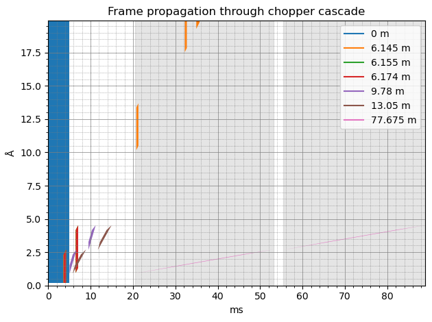
There should be one vertical band matching the extent of each pink polygon, which there is.

Computing a time-of-flight coordinate

We will now use our workflow to obtain our event data with a time-of-flight coordinate:

tofs = workflow.compute(unwrap.TofData)
tofs

scipp.DataArray (4.50 MB)

• Dimensions:
  • pulse: 5
• Coordinates: (1)
  • Ltotal
    ()
    float64
    m
    71.53

    Values:
    array(71.53)

• Data: (1)
  • (pulse)
    DataArrayView
    binned data [len=15633, len=18056, len=17969, len=18179, len=2622]

    dim='event',
    content=DataArray(
              dims=(event: 72459),
              data=float64[counts],
              coords={'id':int64, 'toa':float64[µs], 'event_time_offset':float64[s],
                      'time_offset':float64[s], 'pulse_time':datetime64[µs],
                      'tof':float64[s], 'time_zero':datetime64[µs]},
              masks={'blocked_by_others':bool})

Histogramming the data for a plot should show a profile with 6 bumps that correspond to the frames:

tofs.bins.concat().hist(tof=300).plot()

Converting to wavelength

We can now convert our new time-of-flight coordinate to a neutron wavelength, using tranform_coords:

from scippneutron.conversion.graph.beamline import beamline
from scippneutron.conversion.graph.tof import elastic

# Perform coordinate transformation
graph = {**beamline(scatter=False), **elastic("tof")}
wav_wfm = tofs.transform_coords("wavelength", graph=graph)

# Define wavelength bin edges
wavs = sc.linspace("wavelength", 0.8, 4.6, 201, unit="angstrom")

wav_wfm.hist(wavelength=wavs).sum("pulse").plot()

Comparing to the ground truth

As a consistency check, because we actually know the wavelengths of the neutrons we created, we can compare the true neutron wavelengths to those we computed above.

ground_truth = ess_beamline.model_result["detector"].data.flatten(to="event")
ground_truth = ground_truth[~ground_truth.masks["blocked_by_others"]]

pp.plot(
    {
        "wfm": wav_wfm.hist(wavelength=wavs).sum("pulse"),
        "ground_truth": ground_truth.hist(wavelength=wavs),
    }
)

Multiple detector pixels

It is also possible to compute the neutron time-of-flight for multiple detector pixels at once, where every pixel has different frame bounds (because every pixel is at a different distance from the source).

In our setup, we simply propagate the same neutrons to multiple detector pixels, as if they were not absorbed by the first pixel they meet.

Ltotal = sc.array(dims=['detector_number'], values=[77.675, 76.0], unit='m')
monitors = {
        f"detector{i}": ltot for i, ltot in enumerate(Ltotal)
    }

ess_beamline = FakeBeamlineEss(
    choppers=choppers,
    monitors=monitors,
    run_length=sc.scalar(1 / 14, unit="s") * 4,
    events_per_pulse=200_000,
)

Our raw data has now a detector_number dimension of length 2.

We can plot the neutron event_time_offset for the two detector pixels and see that the offsets are shifted to the left for the pixel that is closest to the source.

raw_data = sc.concat(
        [ess_beamline.get_monitor(key) for key in monitors.keys()],
        dim='detector_number',
    )

# Visualize
pp.plot(sc.collapse(raw_data.hist(event_time_offset=300).sum("pulse"), keep='event_time_offset'))

Computing time-of-flight is done in the same way as above. We need to remember to update our workflow:

# Update workflow
workflow[unwrap.Ltotal] = Ltotal
workflow[unwrap.RawData] = raw_data

# Compute tofs and wavelengths
tofs = workflow.compute(unwrap.TofData)
wav_wfm = tofs.transform_coords("wavelength", graph=graph)

# Compare in plot
ground_truth = []
for det in ess_beamline.monitors:
    data = ess_beamline.model_result[det.name].data.flatten(to="event")
    ground_truth.append(data[~data.masks["blocked_by_others"]])

figs = [
    pp.plot(
        {
            "wfm": wav_wfm['detector_number', i].bins.concat().hist(wavelength=wavs),
            "ground_truth": ground_truth[i].hist(wavelength=wavs),
        }, title=f"Pixel {i+1}"
    ) for i in range(len(Ltotal))
]

figs[0] + figs[1]

Handling time overlap between subframes

In some (relatively rare) cases, where a chopper cascade is slightly ill-defined, it is sometimes possible for some subframes to overlap in time with other subframes.

This is basically when neutrons passed through different pulse-shaping chopper openings, but arrive at the same time at the detector.

In this case, it is actually not possible to accurately determine the wavelength of the neutrons. ScippNeutron handles this by clipping the overlapping regions and throwing away any neutrons that lie within it.

To simulate this, we modify slightly the phase and the cutouts of the band-control chopper:

disk_choppers['bcc'] = DiskChopper(
    frequency=sc.scalar(112.0, unit="Hz"),
    beam_position=sc.scalar(0.0, unit="deg"),
    phase=sc.scalar(240 - 180, unit="deg"),
    axle_position=sc.vector(value=[0, 0, 9.78], unit="m"),
    slit_begin=sc.array(dims=["cutout"], values=[-36.875, 143.125], unit="deg"),
    slit_end=sc.array(dims=["cutout"], values=[46.875, 216.875], unit="deg"),
    slit_height=sc.scalar(10.0, unit="cm"),
    radius=sc.scalar(30.0, unit="cm"),
)


# Update the choppers
choppers = {
    key: chopper_cascade.Chopper.from_disk_chopper(
        chop,
        pulse_frequency=sc.scalar(14.0, unit="Hz"),
        npulses=1,
    )
    for key, chop in disk_choppers.items()
}

# Go back to a single detector pixel
Ltotal = sc.scalar(76.55 + 1.125, unit="m")

ess_beamline = FakeBeamlineEss(
    choppers=choppers,
    monitors={"detector": Ltotal},
    run_length=sc.scalar(1 / 14, unit="s") * 4,
    events_per_pulse=200_000,
)

ess_beamline.model_result.plot()

Plot(ax=<Axes: xlabel='Time-of-flight (us)', ylabel='Distance (m)'>, fig=<Figure size 1200x480 with 2 Axes>)

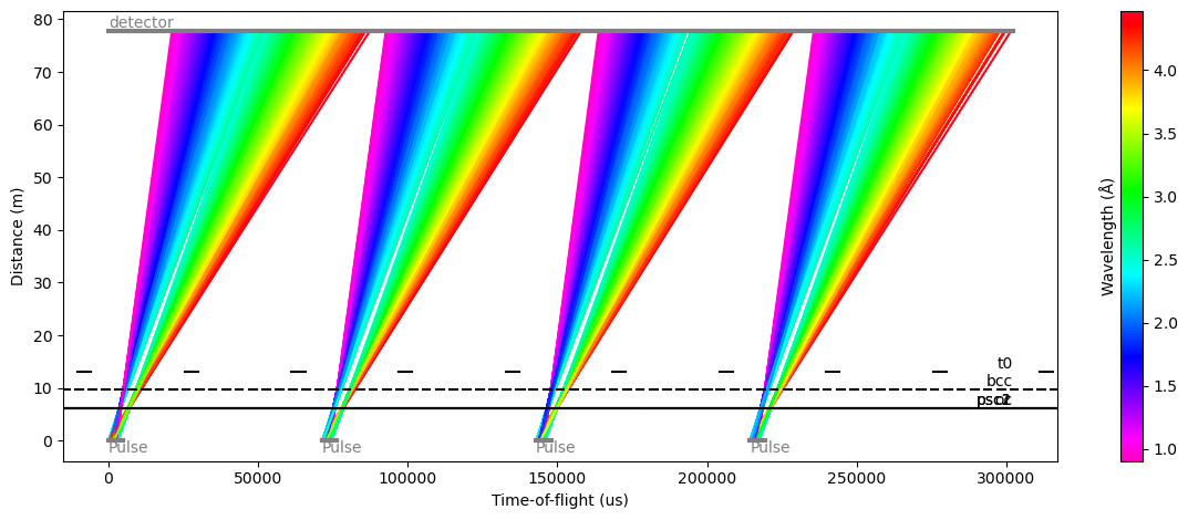
We can now see that there is no longer a gap between the two frames at the center of each pulse (green region).

Another way of looking at this is making the chopper-cascade diagram and zooming in on the last frame (pink), which also show overlap in time:

# Chop the frames
chopped = frames.chop(choppers.values())

# Propagate the neutrons to the detector
at_sample = chopped.propagate_to(Ltotal)

# Visualize the results
cascade_fig, cascade_ax = at_sample.draw()
cascade_ax.set_xlim(45.0, 58.0)
cascade_ax.set_ylim(2.0, 3.0)

(2.0, 3.0)

We now update our workflow with the new choppers and raw data, compute the frame bounds and overlay them on the figure.

workflow[unwrap.Choppers] = choppers
workflow[unwrap.Ltotal] = Ltotal
workflow[unwrap.RawData] = ess_beamline.get_monitor("detector")


bounds = workflow.compute(unwrap.CleanFrameAtDetector).subbounds()

for b in sc.collapse(bounds["time"], keep="bound").values():
    cascade_ax.axvspan(
        b[0].to(unit="ms").value,
        b[1].to(unit="ms").value,
        color="gray",
        alpha=0.2,
        zorder=-5,
    )

cascade_fig

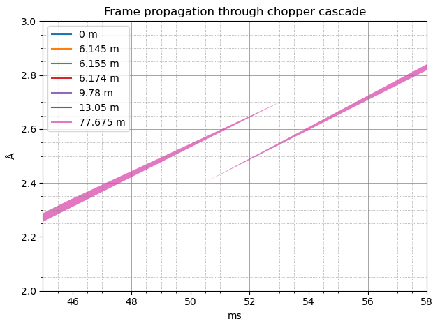
We see that instead of having overlapping bounds, the region in the middle has been excluded.

This means that the neutrons in the overlapping region will be discarded in the time-of-flight calculation (in practice, they are given a NaN value as a time-of-flight).

This is visible when comparing to the true neutron wavelengths, where we see that some counts were lost between the two frames.

# Compute time-of-flight
tofs = workflow.compute(unwrap.TofData)
# Compute wavelength
wav_wfm = tofs.transform_coords("wavelength", graph=graph)

# Compare to the true wavelengths
ground_truth = ess_beamline.model_result["detector"].data.flatten(to="event")
ground_truth = ground_truth[~ground_truth.masks["blocked_by_others"]]

pp.plot(
    {
        "wfm": wav_wfm.hist(wavelength=wavs).sum("pulse"),
        "ground_truth": ground_truth.hist(wavelength=wavs),
    }
)