ESS instruments

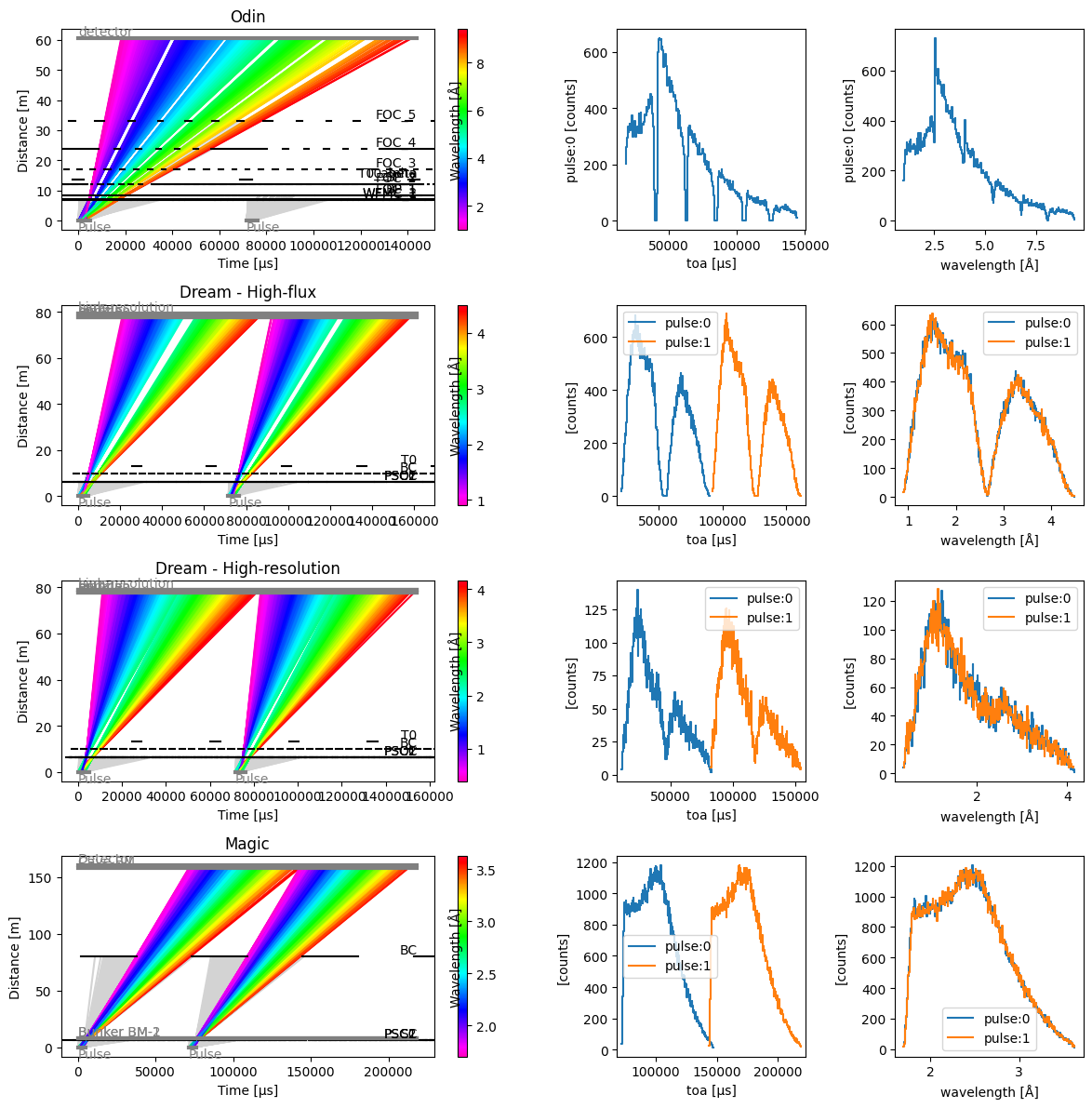
Here we construct a grid of plots showing the chopper cascades of different ESS instruments.

import matplotlib.pyplot as plt
from matplotlib.gridspec import GridSpec
import tof

instruments = {
    # Note that for Odin, we could also use the 'ess-odin' facility when building
    # the Source below
    "Odin": tof.facilities.ess.odin(pulse_skipping=True),
    "Dream - High-flux": tof.facilities.ess.dream(high_flux=True),
    "Dream - High-resolution": tof.facilities.ess.dream(high_resolution=True),
    "Magic": tof.facilities.ess.magic(psc_opening_angle=105, wavelength_band_min=1.8),
}

fig = plt.figure(figsize=(9, 3 * len(instruments)))
gs = GridSpec(nrows=len(instruments), ncols=4, figure=fig)

source = tof.Source(facility="ess", neutrons=1_000_000, pulses=2)

for i, (name, params) in enumerate(instruments.items()):
    model = tof.Model(source=source, **params)
    results = model.run()
    ax1 = fig.add_subplot(gs[i, 0:2])
    ax2 = fig.add_subplot(gs[i, 2])
    ax3 = fig.add_subplot(gs[i, 3])
    results.plot(ax=ax1, blocked_rays=5000)
    ax1.set_title(name)
    furthest_detector = sorted(results.detectors.values(), key=lambda c: c.distance)[-1]
    furthest_detector.toa.plot(ax=ax2)
    furthest_detector.wavelength.plot(ax=ax3)