Demo#

This notebook is a short example on how to use the tof package for making time-of-light diagrams of neutrons passing through a chopper cascade.

[1]:

import scipp as sc
import tof

Hz = sc.Unit('Hz')
deg = sc.Unit('deg')
meter = sc.Unit('m')

Create a source pulse#

We first create a source with one pulse containing 1 million neutrons whose distribution follows the ESS time and wavelength profiles (both thermal and cold neutrons are included).

[2]:

source = tof.Source(facility='ess', neutrons=1_000_000)
source

[2]:

Source:
  pulses=1, neutrons per pulse=1000000
  frequency=14.0 Hz
  facility='ess'

[3]:

source.plot()

[3]:

Chopper set-up#

We create a list of choppers that will be included in our beamline. In our case, we make two WFM choppers, and two frame-overlap choppers. All choppers have 6 openings.

[4]:

choppers = [
    tof.Chopper(
        frequency=70.0 * Hz,
        open=sc.array(
            dims=['cutout'],
            values=[98.71, 155.49, 208.26, 257.32, 302.91, 345.3],
            unit='deg',
        ),
        close=sc.array(
            dims=['cutout'],
            values=[109.7, 170.79, 227.56, 280.33, 329.37, 375.0],
            unit='deg',
        ),
        phase=47.10 * deg,
        distance=6.6 * meter,
        name="WFM1",
    ),
    tof.Chopper(
        frequency=70 * Hz,
        open=sc.array(
            dims=['cutout'],
            values=[80.04, 141.1, 197.88, 250.67, 299.73, 345.0],
            unit='deg',
        ),
        close=sc.array(
            dims=['cutout'],
            values=[91.03, 156.4, 217.18, 269.97, 322.74, 375.0],
            unit='deg',
        ),
        phase=76.76 * deg,
        distance=7.1 * meter,
        name="WFM2",
    ),
    tof.Chopper(
        frequency=56 * Hz,
        open=sc.array(
            dims=['cutout'],
            values=[74.6, 139.6, 194.3, 245.3, 294.8, 347.2],
            unit='deg',
        ),
        close=sc.array(
            dims=['cutout'],
            values=[95.2, 162.8, 216.1, 263.1, 310.5, 371.6],
            unit='deg',
        ),
        phase=62.40 * deg,
        distance=8.8 * meter,
        name="Frame-overlap 1",
    ),
    tof.Chopper(
        frequency=28 * Hz,
        open=sc.array(
            dims=['cutout'],
            values=[98.0, 154.0, 206.8, 254.0, 299.0, 344.65],
            unit='deg',
        ),
        close=sc.array(
            dims=['cutout'],
            values=[134.6, 190.06, 237.01, 280.88, 323.56, 373.76],
            unit='deg',
        ),
        phase=12.27 * deg,
        distance=15.9 * meter,
        name="Frame-overlap 2",
    ),
    tof.Chopper(
        frequency=7 * Hz,
        open=sc.array(
            dims=['cutout'],
            values=[30.0],
            unit='deg',
        ),
        close=sc.array(
            dims=['cutout'],
            values=[140.0],
            unit='deg',
        ),
        phase=0 * deg,
        distance=22 * meter,
        name="Pulse-overlap",
    ),
]

Detector set-up#

We add a monitor 26 meters from the source, and a main detector 32 meters from the source.

[5]:

detectors = [
    tof.Detector(distance=26.0 * meter, name='monitor'),
    tof.Detector(distance=32.0 * meter, name='detector'),
]

Run the model#

We combine the source, choppers, and detectors into our model, and then use the .run() method to execute the ray-tracing simulation.

[6]:

model = tof.Model(source=source, choppers=choppers, detectors=detectors)
model

[6]:

Model:
  Source: Source:
  pulses=1, neutrons per pulse=1000000
  frequency=14.0 Hz
  facility='ess'
  Choppers:
    WFM1: Chopper(name=WFM1, distance=6.6 m, frequency=70.0 Hz, phase=47.1 deg, direction=CLOCKWISE, cutouts=6)
    WFM2: Chopper(name=WFM2, distance=7.1 m, frequency=70.0 Hz, phase=76.76 deg, direction=CLOCKWISE, cutouts=6)
    Frame-overlap 1: Chopper(name=Frame-overlap 1, distance=8.8 m, frequency=56.0 Hz, phase=62.4 deg, direction=CLOCKWISE, cutouts=6)
    Frame-overlap 2: Chopper(name=Frame-overlap 2, distance=15.9 m, frequency=28.0 Hz, phase=12.27 deg, direction=CLOCKWISE, cutouts=6)
    Pulse-overlap: Chopper(name=Pulse-overlap, distance=22.0 m, frequency=7.0 Hz, phase=0.0 deg, direction=CLOCKWISE, cutouts=1)
  Detectors:
    monitor: Detector(name=monitor, distance=26.0 m)
    detector: Detector(name=detector, distance=32.0 m)

[7]:

res = model.run()
res

[7]:

Result:
  Source: 1 pulses, 1000000 neutrons per pulse.
  Choppers:
    WFM1: visible=210808, blocked=789192
    WFM2: visible=126273, blocked=84535
    Frame-overlap 1: visible=102038, blocked=24235
    Frame-overlap 2: visible=73208, blocked=28830
    Pulse-overlap: visible=73152, blocked=56
  Detectors:
    monitor: visible=73152
    detector: visible=73152

Results#

Plotting#

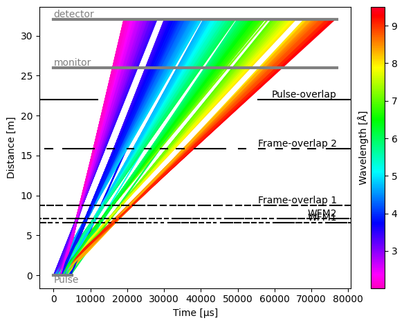
We can plot the models as a whole (which will show the ray paths through the system), and the individual components (which will show the counts each component is seeing).

[8]:

res.plot(visible_rays=5000)

[8]:

Plot(ax=<Axes: xlabel='Time [μs]', ylabel='Distance [m]'>, fig=<Figure size 640x480 with 2 Axes>)

[9]:

res.detectors['monitor'].toa.plot()

[9]:

[10]:

res.choppers["Frame-overlap 2"].toa.plot()

[10]: