WFM#

Wavelength-frame-multiplication (WFM) is a technique commonly used at long-pulse facilities to improve the resolution of the results measured at the neutron detectors. See for example the article by Schmakat et al. (2020) for a description of how WFM works.

In this notebook, we show how tof can be used to convert a neutron time of arrival at the detector to a wavelength.

[1]:

import scipp as sc
import plopp as pp
import tof

Hz = sc.Unit("Hz")
deg = sc.Unit("deg")
meter = sc.Unit("m")

Component set-up#

Choppers#

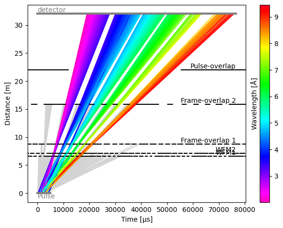
We create a list of choppers that will be included in our beamline. In our case, we make two WFM choppers, and two frame-overlap choppers. All choppers have 6 openings.

Finally, we also add a pulse-overlap chopper with a single opening. These choppers are copied after the V20 ESS beamline at HZB.

[4]:

choppers = [
    tof.Chopper(
        frequency=70.0 * Hz,
        open=sc.array(
            dims=["cutout"],
            values=[98.71, 155.49, 208.26, 257.32, 302.91, 345.3],
            unit="deg",
        ),
        close=sc.array(
            dims=["cutout"],
            values=[109.7, 170.79, 227.56, 280.33, 329.37, 375.0],
            unit="deg",
        ),
        phase=47.10 * deg,
        distance=6.6 * meter,
        name="WFM1",
    ),
    tof.Chopper(
        frequency=70 * Hz,
        open=sc.array(
            dims=["cutout"],
            values=[80.04, 141.1, 197.88, 250.67, 299.73, 345.0],
            unit="deg",
        ),
        close=sc.array(
            dims=["cutout"],
            values=[91.03, 156.4, 217.18, 269.97, 322.74, 375.0],
            unit="deg",
        ),
        phase=76.76 * deg,
        distance=7.1 * meter,
        name="WFM2",
    ),
    tof.Chopper(
        frequency=56 * Hz,
        open=sc.array(
            dims=["cutout"],
            values=[74.6, 139.6, 194.3, 245.3, 294.8, 347.2],
            unit="deg",
        ),
        close=sc.array(
            dims=["cutout"],
            values=[95.2, 162.8, 216.1, 263.1, 310.5, 371.6],
            unit="deg",
        ),
        phase=62.40 * deg,
        distance=8.8 * meter,
        name="Frame-overlap 1",
    ),
    tof.Chopper(
        frequency=28 * Hz,
        open=sc.array(
            dims=["cutout"],
            values=[98.0, 154.0, 206.8, 254.0, 299.0, 344.65],
            unit="deg",
        ),
        close=sc.array(
            dims=["cutout"],
            values=[134.6, 190.06, 237.01, 280.88, 323.56, 373.76],
            unit="deg",
        ),
        phase=12.27 * deg,
        distance=15.9 * meter,
        name="Frame-overlap 2",
    ),
    tof.Chopper(
        frequency=7 * Hz,
        open=sc.array(
            dims=["cutout"],
            values=[30.0],
            unit="deg",
        ),
        close=sc.array(
            dims=["cutout"],
            values=[140.0],
            unit="deg",
        ),
        phase=0 * deg,
        distance=22 * meter,
        name="Pulse-overlap",
    ),
]

Detectors#

We add a single detector 32 meters from the source.

[5]:

detectors = [
    tof.Detector(distance=32.0 * meter, name="detector"),
]

Run the simulation#

We propagate our pulse of neutrons through the chopper cascade and inspect the results.

[6]:

model = tof.Model(source=source, choppers=choppers, detectors=detectors)
results = model.run()
results.plot(blocked_rays=5000)

[6]:

Plot(ax=<Axes: xlabel='Time [μs]', ylabel='Distance [m]'>, fig=<Figure size 640x480 with 2 Axes>)

Wavelength as a function of time-of-arrival#

Plotting wavelength vs time-of-arrival#

Since we know the true wavelength of our neutrons, as well as the time at which the neutrons arrive at the detector (coordinate named toa in the detector reading), we can plot an image of the wavelengths as a function of time-of-arrival:

[7]:

# Squeeze the pulse dimension since we only have one pulse
events = results['detector'].data.squeeze()
# Remove the events that don't make it to the detector
events = events[~events.masks['blocked_by_others']]
# Histogram and plot
events.hist(wavelength=500, toa=500).plot(norm='log', grid=True)

[7]:

Defining a conversion from `toa` to `wavelength`#

The image above shows that there is a pretty tight correlation between time-of-arrival and wavelength.

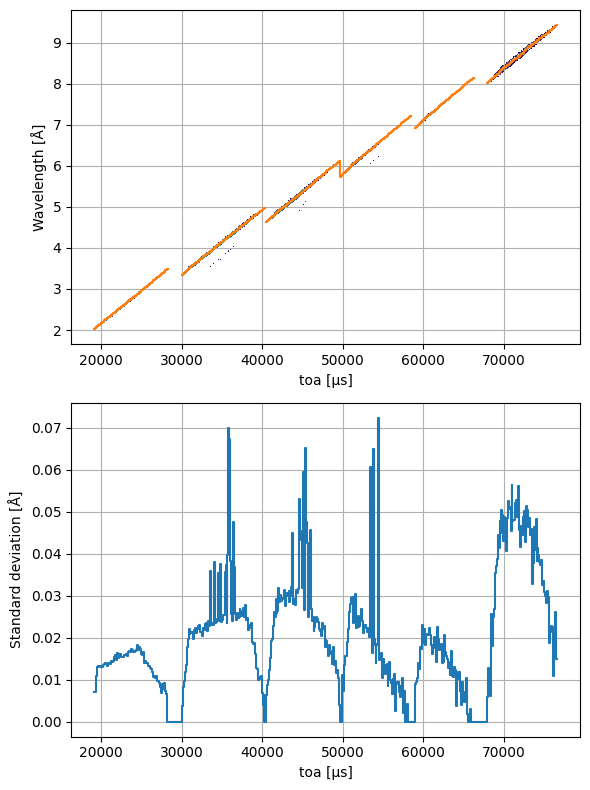
We compute the mean wavelength inside a given toa bin to define a relation between toa and wavelength.

[8]:

binned = events.bin(toa=500)

# Weighted mean of wavelength inside each bin
mu = (
    binned.bins.data * binned.bins.coords['wavelength']
).bins.sum() / binned.bins.sum()

# Variance of wavelengths inside each bin
var = (
    binned.bins.data * (binned.bins.coords['wavelength'] - mu) ** 2
) / binned.bins.sum()

We can now overlay our mean wavelength function on the image above:

[9]:

import matplotlib.pyplot as plt

fig, ax = plt.subplots(2, 1)

f = events.hist(wavelength=500, tof=500).plot(norm='log', cbar=False, ax=ax[0])
mu.name = 'Wavelength'
mu.plot(ax=ax[0], color='C1', grid=True)
stddev = sc.sqrt(var.hist())
stddev.name = 'Standard deviation'
stddev.plot(ax=ax[1], grid=True)
fig.set_size_inches(6, 8)
fig.tight_layout()

Computing wavelengths#

We set up an interpolator that will compute wavelengths given an array of toas.

[10]:

from scipp.scipy.interpolate import interp1d

# Set up interpolator
y = mu.copy()
y.coords['toa'] = sc.midpoints(y.coords['toa'])
f = interp1d(y, 'toa', bounds_error=False)

# Compute wavelengths
wavs = f(events.coords['toa'].rename_dims(event='toa'))
wavelengths = sc.DataArray(
    data=sc.ones(sizes=wavs.sizes, unit='counts'), coords={'wavelength': wavs.data}
).rename_dims(toa='event')
wavelengths

[10]:

scipp.DataArray (570.08 KB)

Dimensions:
- event: 36431

Coordinates: (1)

wavelength

(event)

float64

Å

3.120, 2.577, ..., 5.685, 4.631

Values:
array([3.12009905, 2.57703063, 2.97127603, ..., 5.10171491, 5.68494471,
       4.63079753], shape=(36431,))

Data: (1)

(event)

float64

counts

1.0, 1.0, ..., 1.0, 1.0

Values:
array([1., 1., 1., ..., 1., 1., 1.], shape=(36431,))

We can now compare our computed wavelengths to the true wavelengths of the neutrons. We also include a naive computation of the neutron wavelengths using the toa coordinate directly with the detector distance.

[11]:

naive = events.copy()
speed = detectors[0].distance / naive.coords['toa']
naive.coords['wavelength'] = sc.reciprocal(
    speed * sc.constants.m_n / sc.constants.h
).to(unit='angstrom')

[12]:

pp.plot(
    {
        'naive': naive.hist(wavelength=300),
        'wfm': wavelengths.hist(wavelength=300),
        'original': events.hist(wavelength=300),
    }
)

[12]:

We can see that the WFM estimate clearly outperforms the naive computation.

WFM#

Create a source pulse#

Component set-up#

Choppers#

Detectors#

Run the simulation#

Wavelength as a function of time-of-arrival#

Plotting wavelength vs time-of-arrival#

Defining a conversion from `toa` to `wavelength`#

Computing wavelengths#

Multiple detectors#

Using a range of detectors#

Relation between `toa` and `wavelength` in 2D#

Computing wavelengths with a 2D interpolator#

WFM#

Create a source pulse#

Component set-up#

Choppers#

Detectors#

Run the simulation#

Wavelength as a function of time-of-arrival#

Plotting wavelength vs time-of-arrival#

Defining a conversion from toa to wavelength#

Computing wavelengths#

Multiple detectors#

Using a range of detectors#

Relation between toa and wavelength in 2D#

Computing wavelengths with a 2D interpolator#

Defining a conversion from `toa` to `wavelength`#

Relation between `toa` and `wavelength` in 2D#