Binned Data#

Introduction#

Scipp supports features for binning scattered data.

Terminology

Scipp distinguishes histogrammed data from binned data:

Histogrammed data refers to regular dense arrays of, e.g., floating-point values with an associated bin-edge coordinate.
Binned data refers to the precursor of histogrammed data, i.e., each bin contains a “list” of contributing events or values. Binned data can be converted into a histogram by computing the sum or mean over all events or values in a bin.

Scattered data in the context of binning refers to data values irregularly placed in, e.g., space or time. Binning lets us:

Map a table of position-based data to an X-Y-Z grid.
Map a table of position-based data to an angle such as \(\theta\).
Map event time stamps to time bins.

The key feature here is that binning does not actually histogram or resample data. Data is kept in its original form. Binning provides a wrapper with a coordinate system more adequate for working with the scientific data.

From scattered to binned data#

We outline the underlying concepts based on a simple example. The scattered raw data is represented as a table with meta data for every data point (event):

[1]:

%matplotlib inline
import numpy as np
import matplotlib.pyplot as plt
import scipp as sc

np.random.seed(1)  # Fixed for reproducibility

Consider a list of measurements at various “points” in space. Here we restrict ourselves to the X-Y plane for visualization purposes:

[2]:

N = 50
values = 10 * np.random.rand(N)
table = sc.DataArray(
    data=sc.array(dims=['row'], unit=sc.units.counts, values=values, variances=values),
    coords={
        'position': sc.array(
            dims=['row'], values=[f'site-{i}' for i in range(N)]
        ),
        'x': sc.array(dims=['row'], unit='m', values=np.random.rand(N)),
        'y': sc.array(dims=['row'], unit='m', values=np.random.rand(N)),
    },
)
table

For every point we measured at the auxiliary coordinates 'x' and 'y' give the position in the X-Y plane. These are not dimension-coordinates, since our measurements are not on a 2-D grid, but rather points with an irregular distribution. data is literally a 1-D table of measurements:

[3]:

sc.table(table)

[3]:

Coordinates			Data
position	x [m]	y [m]	[counts]
site-0	0.019	0.327	4.170±2.042
site-1	0.679	0.527	7.203±2.684
site-2	0.212	0.886	0.001±0.034
site-3	0.266	0.357	3.023±1.739
site-4	0.492	0.909	1.468±1.211
site-5	0.053	0.623	0.923±0.961
site-6	0.574	0.016	1.863±1.365
site-7	0.147	0.929	3.456±1.859
site-8	0.589	0.691	3.968±1.992
site-9	0.700	0.997	5.388±2.321
...	...	...	...
site-40	0.115	0.556	9.889±3.145
site-41	0.949	0.136	7.482±2.735
site-42	0.450	0.060	2.804±1.675
site-43	0.578	0.121	7.893±2.809
site-44	0.408	0.045	1.032±1.016
site-45	0.237	0.107	4.479±2.116
site-46	0.903	0.226	9.086±3.014
site-47	0.574	0.713	2.936±1.714
site-48	0.003	0.560	2.878±1.696
site-49	0.617	0.013	1.300±1.140

We can plot this data:

[4]:

table.plot()

[4]:

../../_images/user-guide_binned-data_binned-data_7_0.svg

The 'row' dimension is not a continuous dimension but essentially just a row in our table. In practice, such a figure and this representation of data in general may therefore not be very useful.

As an alternative view of our data we can create a scatter plot. We do this explicitly here to demonstrate how the content of data is connected to elements of the figure:

[5]:

fig, ax = plt.subplots(dpi=96)
scatter = ax.scatter(
    x=table.coords['x'].values, y=table.coords['y'].values, c=table.values
)
ax.set_xlabel('x [{}]'.format(table.coords['x'].unit))
ax.set_ylabel('y [{}]'.format(table.coords['y'].unit))
cbar = plt.colorbar(scatter)
cbar.set_label(f"[{table.unit}]")

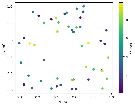
../../_images/user-guide_binned-data_binned-data_9_0.png

This shows the distribution in space, but for real datasets with millions of points this is not practical. Furthermore, operating with scattered data is often inconvenient and may require knowledge of the underlying representation.

We can now use scipp.bin to provide a more accessible wrapper for our data:

[6]:

binned = table.bin(y=4, x=2)
binned

[6]:

scipp.DataArray (5.34 KB)

Dimensions:
- y: 4
- x: 2

Coordinates: (2)

(x [bin-edge])

float64

0.003, 0.484, 0.965

Values:
array([0.00287033, 0.48385519, 0.96484005])

(y [bin-edge])

float64

0.013, 0.259, 0.505, 0.751, 0.997

Values:
array([0.01255598, 0.2587477 , 0.50493942, 0.75113113, 0.99732285])

Data: (1)

(y, x)

DataArrayView

binned data [len=9, len=10, ..., len=6, len=8]

dim='row',
content=DataArray(
          dims=(row: 50),
          data=float64[counts],
          coords={'position':string, 'x':float64[m], 'y':float64[m]})

binned is a 2-D data array, but it contains (a reordered copy) the original table of “unaligned” data. Each element of binned is a view of a section of that table:

[7]:

binned.values[0]

The binning procedure based on bin edges for 'x' and 'y' is not performing the actual histogramming step. However, since its dimensions are defined by the bin-edge coordinates for 'x' and 'y', we will see below that it behaves much like normal dense data for operations such as slicing.

We create another figure to better illustrate the structure of binned:

[8]:

fig, ax = plt.subplots(dpi=96)
buffer = binned.bins.constituents['data']
scatter = ax.scatter(
    x=buffer.coords['x'].values, y=buffer.coords['y'].values, c=buffer.values
)
ax.set_xlabel('x [{}]'.format(binned.coords['x'].unit))
ax.set_ylabel('y [{}]'.format(binned.coords['y'].unit))
ax.set_xticks(binned.coords['x'].values)
ax.set_yticks(binned.coords['y'].values)
ax.grid()
cbar = fig.colorbar(scatter)
cbar.set_label(f"[{table.unit}]")

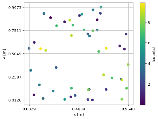
../../_images/user-guide_binned-data_binned-data_15_0.png

This is essentially the same figure as the scatter plot for the original data. The differences are:

A “grid” (the bin edges) that is stored alongside the data.
All points outside the limits of the specified bin edges have been dropped

binned can now directly be histogrammed, without the need for specifying bin boundaries:

[9]:

binned.hist().plot()

[9]:

../../_images/user-guide_binned-data_binned-data_17_0.svg

Note that calling binned.hist() is equivalent to binned.bins.sum(), summing the data array within each bin. Here sum performs histogramming for all “binned” dimensions, in this case x and y. The resulting values in the X-Y bins are the counts accumulated from measurements at all points falling in a given bin.

We can explicitly histogram with a different bin count the binned data for a higher-resolution plot:

[10]:

binned.hist(y=10, x=10).plot()

[10]:

../../_images/user-guide_binned-data_binned-data_19_0.svg

Note

Unless Plopp is used for plotting (as in the Scipp documentation, but not enabled by default yet), plot() will automatically histogram and resample data. Automatic resampling by plot() will be removed in the near future, due to the inconsistent results. In the future explicit binning will be required, and we recommend explicit histogramming already now, to easy the transition in the future.

Working with binned data#

Slicing#

Binned data can be sliced as usual, e.g., to create plots of subregions:

[11]:

binned['x', 0].hist(y=10).plot()

[11]:

../../_images/user-guide_binned-data_binned-data_22_0.svg

Just like slicing dense variables, a slice of binned data “drops” all scattered data falling into areas outside the slice:

[12]:

s0 = binned['x', 0]
s1 = binned['x', 1]
print(f'total events: {binned.sum().value}')
print(f'events x=0:   {s0.sum().value}')
print(f'events x=1:   {s1.sum().value}')

total events: 233.48779981759884
events x=0:   102.78766950179809
events x=1:   130.7001303158007

This can provide an intuitive way of “filtering” lists of data based on some property of the list items.

Masking#

Masks can be defined for the scattered data array, as well as the bin wrapper. This gives fine-grained and intuitive control, for e.g., masking invalid list entries on the one hand, and excluding regions in space on the other hand, without the need of manually determining which list entries fall into the exclusion zone.

We define two masks one in the X-Y plane and one for positions. The position mask is added to the masks dict of the bins property:

[13]:

binned = binned.bin(y=10, x=10)
x_y_mask = (binned.coords['x'][1:] < 0.5 * sc.Unit('m')) & (
    binned.coords['y'][1:] < 0.5 * sc.Unit('m')
)
binned.masks['exclude'] = x_y_mask
binned.bins.masks['broken_sensor'] = binned.bins.coords['y'] > 0.6 * sc.Unit('m')

As usual, more masks can be added if required, and masks can be removed as long as no reduction operation such as summing or histogramming took place.

We can then plot the result. The mask of the underlying scattered data is applied during the histogram step, i.e., masked positions are excluded. The mask of the binned wrapper is indicated in the plot and carried through the histogram step, provided that the binning is not changed. Make sure to compare this figure with the one we obtained earlier, before masking, and note how the values of the un-masked X-Y bins have changed due to masked positions of the underlying unaligned data:

[14]:

binned.hist().plot()

[14]:

../../_images/user-guide_binned-data_binned-data_29_0.svg

Arithmetic operations#

A number of arithmetic operations and other operations for binned data arrays are supported.

Manipulating bin-based and event-based metadata#

Convert bin-based coordinate into event-based coordinate#

Consider binned data as above, but with a coordinate that has no corresponding event-coord. This could be the case, e.g., with a time dimension that corresponds to groups rather than bins:

[15]:

da = table.bin(y=4, x=2)
del da.coords['y']
del da.bins.coords['y']
da = da.rename_dims({'y': 'time'})
da.coords['time'] = sc.arange('time', 4, unit='s')
da

[15]:

scipp.DataArray (4.70 KB)

Dimensions:
- time: 4
- x: 2
Coordinates: (2)
- time
  (time)
  int64
  s
  0, 1, 2, 3
```
Values:
array([0, 1, 2, 3])
```
- x
  (x [bin-edge])
  float64
  m
  0.003, 0.484, 0.965
```
Values:
array([0.00287033, 0.48385519, 0.96484005])
```

Data: (1)

(time, x)

DataArrayView

binned data [len=9, len=10, ..., len=6, len=8]

dim='row',
content=DataArray(
          dims=(row: 50),
          data=float64[counts],
          coords={'position':string, 'x':float64[m]})

If we, e.g., intend to erase the grouping dimension, we may nevertheless want to preserve the time information. This can be achieved using bins_like to broadcast, for each bin, a single value to a “list” of the required size:

[16]:

da.bins.coords['time'] = sc.bins_like(da, da.coords['time'])
sc.table(da.values[0])

[16]:

Coordinates			Data
position	time [s]	x [m]	[counts]
site-10	0	0.102	4.192±2.047
site-11	0	0.414	6.852±2.618
site-14	0	0.050	0.274±0.523
site-21	0	0.137	9.683±3.112
site-22	0	0.139	3.134±1.770
site-33	0	0.349	5.332±2.309
site-42	0	0.450	2.804±1.675
site-44	0	0.408	1.032±1.016
site-45	0	0.237	4.479±2.116

Note the different values for the time coordinate above and below:

[17]:

sc.table(da.values[2])

[17]:

Coordinates			Data
position	time [s]	x [m]	[counts]
site-0	1	0.019	4.170±2.042
site-3	1	0.266	3.023±1.739