Working with masks#
Introduction#
Scipp supports non-destructive masks stored alongside data. In this tutorial we learn how to create and use masks.
This tutorial contains exercises, but solutions are included directly. We encourage you to download this notebook and run through it step by step before looking at the solutions. We recommend to use a recent version of JupyterLab: The solutions are included as hidden cells and shown only on demand.
As a side effect, the exercises will help in getting more familiar with the basic concepts of operations.
First, in addition to importing scipp, we import scippneutron since this is required for loading Nexus files:
[1]:
import scipp as sc
import scippneutron as scn
import scippneutron.data
import numpy as np
We start by loading some data, in this case measured with a prototype of the LoKI detectors at the LARMOR beamline:
[2]:
dg = scn.data.tutorial_dense_data()
dg
[2]:
- detectorscippDataArray(spectrum: 114688, tof: 200)float64counts0.0, 0.0, ..., 0.0, 0.0
- scippDataGroup(tof: 200)
- monitor1scippDataArray(tof: 200)float64counts583.995, 112.997, ..., 75.196, 4036.448
- monitor2scippDataArray(tof: 200)float64counts45.997, 42.998, ..., 46.849, 36.547
- monitor3scippDataArray(tof: 200)float64counts0.0, 0.0, ..., 0.0, 0.0
- monitor4scippDataArray(tof: 200)float64counts359.964, 502.005, ..., 50.146, 71.448
- monitor5scippDataArray(tof: 200)float64counts0.0, 0.0, ..., 0.0, 0.0
- proton_charge_by_periodscippVariable()float64𝟙0.3437764048576355
- gd_prtn_chrgscippVariable()float64𝟙2.750211238861084
- DCMagField1scippDataArray(time: 24)float64𝟙-0.002, -0.002, ..., -0.002, -0.002
- DCMagField2scippDataArray(time: 24)float64𝟙0.0, 0.0, ..., 0.0, 0.0
- DCMagField3scippDataArray(time: 24)float64𝟙-1.085, -1.085, ..., -1.085, -1.085
- DCMagField4scippDataArray(time: 24)float64𝟙-1.752, -1.752, ..., -1.752, -1.752
- instrument_namestr()LARMOR
- run_endstr()2019-12-18T18:36:41
- run_startstr()2019-12-18T17:36:11
- run_headerstr()LAR 49293 Dalgliesh,Raspino,Ho LOKI Detector Test Dumm 16-DEC-2019 17:53:49 ...
- run_statusscippDataArray(time: 2)int32𝟙1, 1
- run_numberstr()49338
[3]:
data = dg['detector'] # the actual measured counts
counts = data.sum('tof') # used later
data
[3]:
- spectrum: 114688
- tof: 200
- position(spectrum)vector3m[ 0.778 0.13046651 29.85877813], [ 0.77506458 0.13046651 29.85877813], ..., [-5.69651663e-01 -2.28657089e-02 2.99532831e+01], [-5.72000000e-01 -2.28657089e-02 2.99532831e+01]
Values:
array([[ 7.78000000e-01, 1.30466508e-01, 2.98587781e+01], [ 7.75064579e-01, 1.30466508e-01, 2.98587781e+01], [ 7.72129159e-01, 1.30466508e-01, 2.98587781e+01], ..., [-5.67303327e-01, -2.28657089e-02, 2.99532831e+01], [-5.69651663e-01, -2.28657089e-02, 2.99532831e+01], [-5.72000000e-01, -2.28657089e-02, 2.99532831e+01]]) - sample_position()vector3m[ 0. 0. 25.3]
Values:
array([ 0. , 0. , 25.3]) - source_position()vector3m[0. 0. 0.]
Values:
array([0., 0., 0.]) - spectrum(spectrum)int32𝟙11, 12, ..., 114697, 114698
Values:
array([ 11, 12, 13, ..., 114696, 114697, 114698], dtype=int32) - tof(tof [bin-edge])float64µs5.0, 504.975, ..., 9.950e+04, 1.000e+05
Values:
array([5.0000000e+00, 5.0497500e+02, 1.0049500e+03, 1.5049250e+03, 2.0049000e+03, 2.5048750e+03, 3.0048500e+03, 3.5048250e+03, 4.0048000e+03, 4.5047750e+03, 5.0047500e+03, 5.5047250e+03, 6.0047000e+03, 6.5046750e+03, 7.0046500e+03, 7.5046250e+03, 8.0046000e+03, 8.5045750e+03, 9.0045500e+03, 9.5045250e+03, 1.0004500e+04, 1.0504475e+04, 1.1004450e+04, 1.1504425e+04, 1.2004400e+04, 1.2504375e+04, 1.3004350e+04, 1.3504325e+04, 1.4004300e+04, 1.4504275e+04, 1.5004250e+04, 1.5504225e+04, 1.6004200e+04, 1.6504175e+04, 1.7004150e+04, 1.7504125e+04, 1.8004100e+04, 1.8504075e+04, 1.9004050e+04, 1.9504025e+04, 2.0004000e+04, 2.0503975e+04, 2.1003950e+04, 2.1503925e+04, 2.2003900e+04, 2.2503875e+04, 2.3003850e+04, 2.3503825e+04, 2.4003800e+04, 2.4503775e+04, 2.5003750e+04, 2.5503725e+04, 2.6003700e+04, 2.6503675e+04, 2.7003650e+04, 2.7503625e+04, 2.8003600e+04, 2.8503575e+04, 2.9003550e+04, 2.9503525e+04, 3.0003500e+04, 3.0503475e+04, 3.1003450e+04, 3.1503425e+04, 3.2003400e+04, 3.2503375e+04, 3.3003350e+04, 3.3503325e+04, 3.4003300e+04, 3.4503275e+04, 3.5003250e+04, 3.5503225e+04, 3.6003200e+04, 3.6503175e+04, 3.7003150e+04, 3.7503125e+04, 3.8003100e+04, 3.8503075e+04, 3.9003050e+04, 3.9503025e+04, 4.0003000e+04, 4.0502975e+04, 4.1002950e+04, 4.1502925e+04, 4.2002900e+04, 4.2502875e+04, 4.3002850e+04, 4.3502825e+04, 4.4002800e+04, 4.4502775e+04, 4.5002750e+04, 4.5502725e+04, 4.6002700e+04, 4.6502675e+04, 4.7002650e+04, 4.7502625e+04, 4.8002600e+04, 4.8502575e+04, 4.9002550e+04, 4.9502525e+04, 5.0002500e+04, 5.0502475e+04, 5.1002450e+04, 5.1502425e+04, 5.2002400e+04, 5.2502375e+04, 5.3002350e+04, 5.3502325e+04, 5.4002300e+04, 5.4502275e+04, 5.5002250e+04, 5.5502225e+04, 5.6002200e+04, 5.6502175e+04, 5.7002150e+04, 5.7502125e+04, 5.8002100e+04, 5.8502075e+04, 5.9002050e+04, 5.9502025e+04, 6.0002000e+04, 6.0501975e+04, 6.1001950e+04, 6.1501925e+04, 6.2001900e+04, 6.2501875e+04, 6.3001850e+04, 6.3501825e+04, 6.4001800e+04, 6.4501775e+04, 6.5001750e+04, 6.5501725e+04, 6.6001700e+04, 6.6501675e+04, 6.7001650e+04, 6.7501625e+04, 6.8001600e+04, 6.8501575e+04, 6.9001550e+04, 6.9501525e+04, 7.0001500e+04, 7.0501475e+04, 7.1001450e+04, 7.1501425e+04, 7.2001400e+04, 7.2501375e+04, 7.3001350e+04, 7.3501325e+04, 7.4001300e+04, 7.4501275e+04, 7.5001250e+04, 7.5501225e+04, 7.6001200e+04, 7.6501175e+04, 7.7001150e+04, 7.7501125e+04, 7.8001100e+04, 7.8501075e+04, 7.9001050e+04, 7.9501025e+04, 8.0001000e+04, 8.0500975e+04, 8.1000950e+04, 8.1500925e+04, 8.2000900e+04, 8.2500875e+04, 8.3000850e+04, 8.3500825e+04, 8.4000800e+04, 8.4500775e+04, 8.5000750e+04, 8.5500725e+04, 8.6000700e+04, 8.6500675e+04, 8.7000650e+04, 8.7500625e+04, 8.8000600e+04, 8.8500575e+04, 8.9000550e+04, 8.9500525e+04, 9.0000500e+04, 9.0500475e+04, 9.1000450e+04, 9.1500425e+04, 9.2000400e+04, 9.2500375e+04, 9.3000350e+04, 9.3500325e+04, 9.4000300e+04, 9.4500275e+04, 9.5000250e+04, 9.5500225e+04, 9.6000200e+04, 9.6500175e+04, 9.7000150e+04, 9.7500125e+04, 9.8000100e+04, 9.8500075e+04, 9.9000050e+04, 9.9500025e+04, 1.0000000e+05])
- (spectrum, tof)float64counts0.0, 0.0, ..., 0.0, 0.0σ = 0.0, 0.0, ..., 0.0, 0.0
Values:
array([[0., 0., 0., ..., 0., 0., 0.], [0., 0., 0., ..., 0., 0., 0.], [0., 0., 0., ..., 0., 0., 0.], ..., [0., 0., 0., ..., 0., 0., 0.], [0., 0., 0., ..., 0., 0., 0.], [0., 0., 0., ..., 0., 0., 0.]])
Variances (σ²):
array([[0., 0., 0., ..., 0., 0., 0.], [0., 0., 0., ..., 0., 0., 0.], [0., 0., 0., ..., 0., 0., 0.], ..., [0., 0., 0., ..., 0., 0., 0.], [0., 0., 0., ..., 0., 0., 0.], [0., 0., 0., ..., 0., 0., 0.]])
Note that the exercises in the following are fictional and do not represent the actual SANS data reduction workflow.
Masks are variables with dtype=bool, stored in the masks dict of a data array. The result of comparison between variables can thus be used as masks:
[4]:
data.coords['spectrum'] < sc.scalar(100)
[4]:
- (spectrum: 114688)boolTrue, True, ..., False, False
Values:
array([ True, True, True, ..., False, False, False])
Exercise 1: Masking a prompt pulse#
Create a prompt-pulse mask for the region between \(17500~\mathrm{\mu s}\) and \(19000~\mathrm{\mu s}\). Notes:
Define, e.g.,
prompt_start = 17500 * sc.Unit('us')and the same for the upper bound of the prompt pulse.Use comparison operators such as
==,<=or>.Combine multiple conditions into one using
&(“and”),|(“or”), or^(“exclusive or”).Masks are stored in a data array by storing them in the
masksdictionary, e.g.,data.masks['prompt-pulse'] = ....If something goes wrong, masks can be removed with Python’s
del, e.g.,del data.masks['wrong'].If you run into an error regarding a length mismatch when inserting the coordinate, remember that
'tof'is a bin-edge coordinate, i.e., it is by 1 longer than the number of bins. Use, e.g., only the left bin edges, i.e., all but the last, to create the masks. This can be achieved using slicing, e.g.,array[dim_name, start_index:end_index].
Use the HTML view and plot the data after masking to explore the effect.
Pass a
dictcontainingcounts(computed above ascounts = data.sum('tof')) and the equivalent counts computed after masking tosc.plot. Use this to verify that the prompt-pulse mask results in removal of counts.
Solution#
[5]:
prompt_start = 17500 * sc.Unit('us')
prompt_stop = 19000 * sc.Unit('us')
tof = data.coords['tof']
mask = (tof['tof', :-1] > prompt_start) & (tof['tof', :-1] < prompt_stop)
data.masks['prompt-pulse'] = mask
data
[5]:
- spectrum: 114688
- tof: 200
- position(spectrum)vector3m[ 0.778 0.13046651 29.85877813], [ 0.77506458 0.13046651 29.85877813], ..., [-5.69651663e-01 -2.28657089e-02 2.99532831e+01], [-5.72000000e-01 -2.28657089e-02 2.99532831e+01]
Values:
array([[ 7.78000000e-01, 1.30466508e-01, 2.98587781e+01], [ 7.75064579e-01, 1.30466508e-01, 2.98587781e+01], [ 7.72129159e-01, 1.30466508e-01, 2.98587781e+01], ..., [-5.67303327e-01, -2.28657089e-02, 2.99532831e+01], [-5.69651663e-01, -2.28657089e-02, 2.99532831e+01], [-5.72000000e-01, -2.28657089e-02, 2.99532831e+01]]) - sample_position()vector3m[ 0. 0. 25.3]
Values:
array([ 0. , 0. , 25.3]) - source_position()vector3m[0. 0. 0.]
Values:
array([0., 0., 0.]) - spectrum(spectrum)int32𝟙11, 12, ..., 114697, 114698
Values:
array([ 11, 12, 13, ..., 114696, 114697, 114698], dtype=int32) - tof(tof [bin-edge])float64µs5.0, 504.975, ..., 9.950e+04, 1.000e+05
Values:
array([5.0000000e+00, 5.0497500e+02, 1.0049500e+03, 1.5049250e+03, 2.0049000e+03, 2.5048750e+03, 3.0048500e+03, 3.5048250e+03, 4.0048000e+03, 4.5047750e+03, 5.0047500e+03, 5.5047250e+03, 6.0047000e+03, 6.5046750e+03, 7.0046500e+03, 7.5046250e+03, 8.0046000e+03, 8.5045750e+03, 9.0045500e+03, 9.5045250e+03, 1.0004500e+04, 1.0504475e+04, 1.1004450e+04, 1.1504425e+04, 1.2004400e+04, 1.2504375e+04, 1.3004350e+04, 1.3504325e+04, 1.4004300e+04, 1.4504275e+04, 1.5004250e+04, 1.5504225e+04, 1.6004200e+04, 1.6504175e+04, 1.7004150e+04, 1.7504125e+04, 1.8004100e+04, 1.8504075e+04, 1.9004050e+04, 1.9504025e+04, 2.0004000e+04, 2.0503975e+04, 2.1003950e+04, 2.1503925e+04, 2.2003900e+04, 2.2503875e+04, 2.3003850e+04, 2.3503825e+04, 2.4003800e+04, 2.4503775e+04, 2.5003750e+04, 2.5503725e+04, 2.6003700e+04, 2.6503675e+04, 2.7003650e+04, 2.7503625e+04, 2.8003600e+04, 2.8503575e+04, 2.9003550e+04, 2.9503525e+04, 3.0003500e+04, 3.0503475e+04, 3.1003450e+04, 3.1503425e+04, 3.2003400e+04, 3.2503375e+04, 3.3003350e+04, 3.3503325e+04, 3.4003300e+04, 3.4503275e+04, 3.5003250e+04, 3.5503225e+04, 3.6003200e+04, 3.6503175e+04, 3.7003150e+04, 3.7503125e+04, 3.8003100e+04, 3.8503075e+04, 3.9003050e+04, 3.9503025e+04, 4.0003000e+04, 4.0502975e+04, 4.1002950e+04, 4.1502925e+04, 4.2002900e+04, 4.2502875e+04, 4.3002850e+04, 4.3502825e+04, 4.4002800e+04, 4.4502775e+04, 4.5002750e+04, 4.5502725e+04, 4.6002700e+04, 4.6502675e+04, 4.7002650e+04, 4.7502625e+04, 4.8002600e+04, 4.8502575e+04, 4.9002550e+04, 4.9502525e+04, 5.0002500e+04, 5.0502475e+04, 5.1002450e+04, 5.1502425e+04, 5.2002400e+04, 5.2502375e+04, 5.3002350e+04, 5.3502325e+04, 5.4002300e+04, 5.4502275e+04, 5.5002250e+04, 5.5502225e+04, 5.6002200e+04, 5.6502175e+04, 5.7002150e+04, 5.7502125e+04, 5.8002100e+04, 5.8502075e+04, 5.9002050e+04, 5.9502025e+04, 6.0002000e+04, 6.0501975e+04, 6.1001950e+04, 6.1501925e+04, 6.2001900e+04, 6.2501875e+04, 6.3001850e+04, 6.3501825e+04, 6.4001800e+04, 6.4501775e+04, 6.5001750e+04, 6.5501725e+04, 6.6001700e+04, 6.6501675e+04, 6.7001650e+04, 6.7501625e+04, 6.8001600e+04, 6.8501575e+04, 6.9001550e+04, 6.9501525e+04, 7.0001500e+04, 7.0501475e+04, 7.1001450e+04, 7.1501425e+04, 7.2001400e+04, 7.2501375e+04, 7.3001350e+04, 7.3501325e+04, 7.4001300e+04, 7.4501275e+04, 7.5001250e+04, 7.5501225e+04, 7.6001200e+04, 7.6501175e+04, 7.7001150e+04, 7.7501125e+04, 7.8001100e+04, 7.8501075e+04, 7.9001050e+04, 7.9501025e+04, 8.0001000e+04, 8.0500975e+04, 8.1000950e+04, 8.1500925e+04, 8.2000900e+04, 8.2500875e+04, 8.3000850e+04, 8.3500825e+04, 8.4000800e+04, 8.4500775e+04, 8.5000750e+04, 8.5500725e+04, 8.6000700e+04, 8.6500675e+04, 8.7000650e+04, 8.7500625e+04, 8.8000600e+04, 8.8500575e+04, 8.9000550e+04, 8.9500525e+04, 9.0000500e+04, 9.0500475e+04, 9.1000450e+04, 9.1500425e+04, 9.2000400e+04, 9.2500375e+04, 9.3000350e+04, 9.3500325e+04, 9.4000300e+04, 9.4500275e+04, 9.5000250e+04, 9.5500225e+04, 9.6000200e+04, 9.6500175e+04, 9.7000150e+04, 9.7500125e+04, 9.8000100e+04, 9.8500075e+04, 9.9000050e+04, 9.9500025e+04, 1.0000000e+05])
- (spectrum, tof)float64counts0.0, 0.0, ..., 0.0, 0.0σ = 0.0, 0.0, ..., 0.0, 0.0
Values:
array([[0., 0., 0., ..., 0., 0., 0.], [0., 0., 0., ..., 0., 0., 0.], [0., 0., 0., ..., 0., 0., 0.], ..., [0., 0., 0., ..., 0., 0., 0.], [0., 0., 0., ..., 0., 0., 0.], [0., 0., 0., ..., 0., 0., 0.]])
Variances (σ²):
array([[0., 0., 0., ..., 0., 0., 0.], [0., 0., 0., ..., 0., 0., 0.], [0., 0., 0., ..., 0., 0., 0.], ..., [0., 0., 0., ..., 0., 0., 0.], [0., 0., 0., ..., 0., 0., 0.], [0., 0., 0., ..., 0., 0., 0.]])
- prompt-pulse(tof)boolFalse, False, ..., False, False
Values:
array([False, False, False, False, False, False, False, False, False, False, False, False, False, False, False, False, False, False, False, False, False, False, False, False, False, False, False, False, False, False, False, False, False, False, False, True, True, True, False, False, False, False, False, False, False, False, False, False, False, False, False, False, False, False, False, False, False, False, False, False, False, False, False, False, False, False, False, False, False, False, False, False, False, False, False, False, False, False, False, False, False, False, False, False, False, False, False, False, False, False, False, False, False, False, False, False, False, False, False, False, False, False, False, False, False, False, False, False, False, False, False, False, False, False, False, False, False, False, False, False, False, False, False, False, False, False, False, False, False, False, False, False, False, False, False, False, False, False, False, False, False, False, False, False, False, False, False, False, False, False, False, False, False, False, False, False, False, False, False, False, False, False, False, False, False, False, False, False, False, False, False, False, False, False, False, False, False, False, False, False, False, False, False, False, False, False, False, False, False, False, False, False, False, False, False, False, False, False, False, False])
[6]:
data.hist(spectrum=500).transpose().plot()
[6]:

[7]:
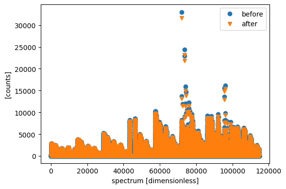
tof = data.coords['tof']
sc.plot({'before': counts, 'after': data.sum('tof')})
[7]:
Exercise 2: Masking spatially#
By masking an x range, mask the end of the tubes.
Define
x = data.coords['position'].fields.xto extract only the x-component of the position coordinate.Create the masks.
Use the instrument view (
scn.instrument_view(data)) to inspect the result.
Solution#
[8]:
x = data.coords['position'].fields.x
data.masks['tube-ends'] = sc.abs(x) > 0.5 * sc.Unit('m')
scn.instrument_view(sc.sum(data, 'tof'), norm='log') # norm='log' is optional
[8]:
Exercise 3: Combining conditions#
Mask the broken pixels with zero counts near the beam stop (center).
Note that there are pixels at larger scattering angles (larger x) which have real zeros. These should not be masked.
Combine the condition for zero counts with a spatial mask, e.g., based on
x, to ensure the mask takes only effect close to the direct beam / beam stop.
[9]:
# This would mask too much, what needs to be added?
counts.data == 0.0 * sc.Unit('counts')
[9]:
- (spectrum: 114688)boolTrue, True, ..., False, True
Values:
array([ True, True, True, ..., False, False, True])
Solution#
[10]:
broken = (counts.data == 0.0 * sc.Unit('counts')) & (sc.abs(x) < 0.1 * sc.Unit('m'))
data.masks['bad-pixels'] = broken
scn.instrument_view(sc.sum(data, 'tof'))
[10]:
Exercise 4: More spatial masking#
Pick one (or more, if desired):
Mask a “circle” (in \(x\)-\(y\) plane, i.e., a cylinder aligned with \(\hat z\))
Mask a ring based on \(x\) and \(y\)
Mask a scattering-angle (\(\theta\)) range. Hint: The scattering angle can be computed as
theta = 0.5 * scn.two_theta(data)Mask a wedge. Hint:
phi = sc.atan2(y=y,x=x)
Solution#
[11]:
pos = data.coords['position']
x = pos.fields.x
y = pos.fields.y
z = pos.fields.z
# could use offsets x0 and y0 to mask away from z axis
r = sc.sqrt(x * x + y * y)
data.masks['circle'] = r < 0.09 * sc.units.m
data.masks['ring'] = (0.14 * sc.units.m < r) & (r < 0.19 * sc.units.m)
theta = 0.5 * scn.two_theta(data)
data.masks['theta'] = (0.03 * sc.units.rad < theta) & (theta < 0.04 * sc.units.rad)
# sc.to_unit is optional, but useful if we prefer degrees rather than radians
phi = sc.to_unit(sc.atan2(y=y, x=x), unit='deg')
data.masks['wedge'] = (10.0 * sc.units.deg < phi) & (phi < 20.0 * sc.units.deg)
scn.instrument_view(sc.sum(data, 'tof'), norm='log')
[11]:
Masks in (grouped) reduction operations#
Finally, let us group according to scattering angle and sum spectra. Questions:
Can you see the effect of the circle/ring/theta-range that you masked above?
Why is the prompt-pulse mask preserved, but not the other masks?
[12]:
theta_edges = sc.array(dims=['theta'], unit='rad', values=np.linspace(0, 0.1, num=100))
data.coords['theta'] = 0.5 * scn.two_theta(data)
data.groupby(group='theta', bins=theta_edges).sum('spectrum').plot()
[12]:

Solution#
The prompt-pulse mask is preserved since we did not sum over time-of-flight.
Masked pixels (spectra) cannot be preserved since we sum over spectra, and the sum simply skips the masked spectra.