Exploring data#

When working with a dataset, the first step is usually to understand what data and metadata it contains. In this chapter we explore how Scipp supports this.

This tutorial contains exercises, but solutions are included directly. We encourage you to download this notebook and run through it step by step before looking at the solutions. We recommend to use a recent version of JupyterLab: The solutions are included as hidden cells and shown only on demand.

First, in addition to importing scipp, we import scippneutron for neutron-science routines.

[1]:

import scipp as sc
import scippneutron as scn
import plopp as pp

We start by loading some data, in this case measured with a prototype of the LoKI detectors at the LARMOR beamline:

[2]:

data = scn.data.tutorial_dense_data()

Downloading file 'loki-at-larmor-filtered.hdf5' from 'https://public.esss.dk/groups/scipp/scippneutron/5/loki-at-larmor-filtered.hdf5' to '/home/runner/.cache/scippneutron/5'.

In practice, we would use scippneutron.load_with_mantid or scippneutron.load_nexus to load the data from a NeXus file, but the tutorial data comes bundled with ScippNeutron to make it easily available. See Tutorial and Test Data for a way to customize where the data is stored.

Note that the exercises in the following are fictional and do not represent the actual SANS data reduction workflow.

Step 2: Plot the data#

Scipp objects (variables, data arrays, datasets, or data groups) can be plotted using the plot() method. Alternatively sc.plot(obj) can be used, e.g., when obj is a Python dict of scipp data arrays. Since this is neutron-scattering data, we can also use the “instrument view”, provided by scn.instrument_view(obj) (assuming scippneutron was imported as scn).

Exercise#

Plot the loaded data and familiarize yourself with the controls.
Create the instrument view and familiarize yourself with the controls.

Solution#

[5]:

detector.sum('spectrum').plot()

[5]:

../_images/tutorials_1_exploring-data_10_0.svg

[6]:

scn.instrument_view(detector.sum('tof'), norm='log')

[6]:

Step 3: Exploring metadata#

Above we saw that the input data group contains a number of metadata items in addition to the the main ‘detector’. Some items are simple strings while others are data arrays or variables. These have various meanings and we now want to explore them.

Exercise#

Find some data array items of data and plot them. Also try sc.table(item) to show a table representation (where item is an item of your choice).
Find and plot a monitor.
Try to normalize detector to monitor 1. Why does this fail?
Plot all the monitors on the same plot. Note that sc.plot() can be used with a data group.

Convert all the monitors from 'tof' to 'wavelength' using, e.g.,

wavelength_graph_monitor = {
    **scn.conversion.graph.beamline.beamline(scatter=False),
    **scn.conversion.graph.tof.elastic_wavelength('tof'),
}
mon1_wav = mon1.transform_coords('wavelength', graph=wavelength_graph_monitor)

Inspect the HTML view and note how the “unit conversion” changed the dimensions and units.
Re-plot all the monitors on the same plot, now in 'wavelength'.

Solution#

[7]:

sc.table(data['DCMagField2'])

[7]:

Coordinates	Data
time [ns]	[𝟙]
2019-12-16T17:53:14.000000000	0.000
2019-12-16T17:53:14.000000000	0.000
2019-12-16T17:53:14.000000000	0.000
2019-12-16T17:53:14.000000000	0.000
2019-12-16T17:53:14.000000000	0.000
2019-12-16T17:53:14.000000000	0.000
2019-12-16T17:53:14.000000000	0.000
2019-12-16T17:53:14.000000000	0.000
2019-12-16T17:53:51.000000000	0.000
2019-12-16T17:53:51.000000000	0.000
...	...
2019-12-16T17:53:51.000000000	0.000
2019-12-16T17:53:51.000000000	0.000
2019-12-18T11:11:16.000000000	0.000
2019-12-18T18:36:41.000000000	0.000
2019-12-19T01:11:41.000000000	0.000
2019-12-19T06:22:07.000000000	0.000
2019-12-19T12:14:46.000000000	0.000
2019-12-19T17:18:58.000000000	0.000
2019-12-19T22:22:32.000000000	0.000
2019-12-20T03:26:14.000000000	0.000

[8]:

detector / data['monitors']['monitor1']

---------------------------------------------------------------------------
DatasetError                              Traceback (most recent call last)
Cell In[8], line 1
----> 1 detector / data['monitors']['monitor1']

DatasetError: Mismatch in coordinate 'position' in operation 'divide':
(spectrum: 114688)    vector3              [m]  [(0.778, 0.130467, 29.8588), (0.775065, 0.130467, 29.8588), ..., (-0.569652, -0.0228657, 29.9533), (-0.572, -0.0228657, 29.9533)]
vs
()    vector3              [m]  (0, 0, 9.8195)

A monitor can be converted to wavelength as follows:

[9]:

wavelength_graph_monitor = {
    **scn.conversion.graph.beamline.beamline(scatter=False),
    **scn.conversion.graph.tof.elastic_wavelength('tof'),
}

[10]:

mon1 = data['monitors']['monitor1']
mon1.transform_coords('wavelength', graph=wavelength_graph_monitor)

[11]:

sc.plot(data['monitors'], norm='log')

[11]:

../_images/tutorials_1_exploring-data_19_0.svg

[12]:

converted_monitors = {
    f'monitor{i}': data['monitors'][f'monitor{i}'].transform_coords(
        'wavelength', graph=wavelength_graph_monitor
    )
    for i in [1, 2, 3, 4, 5]
}
sc.plot(converted_monitors, norm='log')

[12]:

../_images/tutorials_1_exploring-data_20_0.svg

Step 5: A closer look at the data#

In the very first task, we summed the data along the spectrum dimension before plotting, yielding a pixel-integrated time-of-flight spectrum of the data. Here, we sum along the tof dimension to inspect the contents of individual pixels:

[16]:

counts = detector.sum('tof')

Exercise#

Create a plot of counts and also try the instrument view.
How many counts are there in total, in all spectra combined?
Plot a single spectrum of detector as a 1-D plot using the slicing syntax array[dim_name, integer_index] to access the spectrum.

Solution#

[17]:

# slice is optional, making plot more readable in the documentation
counts['spectrum', 56000:62000].plot()

[17]:

../_images/tutorials_1_exploring-data_31_0.svg

[18]:

scn.instrument_view(counts, norm='log')

[18]:

[19]:

# detector.sum('spectrum') # would be another solution
detector.sum().value

[19]:

58142417.0

[20]:

detector['spectrum', 10000].plot()

[20]:

../_images/tutorials_1_exploring-data_34_0.svg

Volumetric detectors#

As seen in the instrument view the detectors consist of 4 layers of tubes, each containing 7 straws. Let us try to split up our data, so we can compare layers. There are other (and probably better) ways to do this, but here we try to define an integer variable containing a layer index:

[21]:

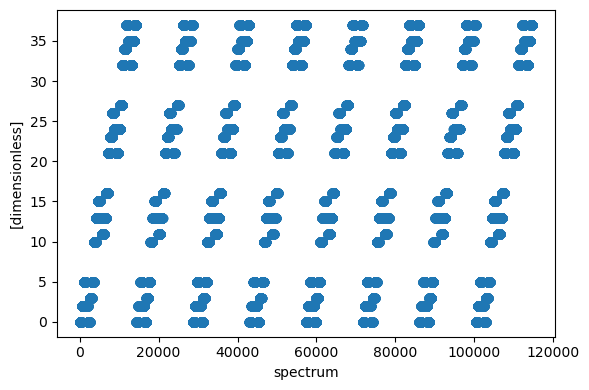
z = detector.coords['position'].fields.z
near = z.min()
far = z.max()
layer = ((z - near) * 400).astype('int32')
layer.unit = ''
layer.plot()

[21]:

../_images/tutorials_1_exploring-data_36_0.png

Exercise#

Change the magic parameter 400 in the cell above until pixels fall cleanly into layers, either 4 layers of tubes or 12 layers of straws.
Store layer as a new coord in detector.
Use detector.groupby(group='layer').sum('spectrum') to group spectra into layers.
Inspect and understand the HTML view of the result.
Plot the result. There are two options:
- Use Plopp’s ``slicer` utility <https://scipp.github.io/plopp/basics/slicer-plot.html>`__ to navigate the different layers using a slider (requires %matplotlib widget to enable interactive figures)
- Use sc.plot after collapsing dimensions, sc.collapse(grouped, keep='tof')
Bonus: When grouping by straw layers, there is a different number of straws in the center layer of each tube (3 instead of 2) due to the flower-pattern arrangement of straws. Define a helper data array with data set to 1 for each spectrum (using, e.g., norm = sc.DataArray(data=sc.ones_like(layer), coords={'layer':layer})), group by layers and sum over spectrum as above, and use this result to normalize the layer-grouped data from above to spectrum count.

Solution#

[22]:

%matplotlib widget
# NOTE:
# - set magic factor to, e.g., 150 to group by straw layer
# - set magic factor to, e.g., 40 to group by tube layer
layer = ((z - near) * 150).astype(sc.DType.int32)
layer.unit = ''
detector.coords['layer'] = layer
grouped = detector.groupby(group='layer').sum('spectrum')
pp.slicer(grouped)

[22]:

[23]:

sc.plot(sc.collapse(grouped, keep='tof'))

[23]:

[24]:

norm = sc.DataArray(data=sc.ones_like(layer), coords={'layer': layer})
norm = norm.groupby(group='layer').sum('spectrum')
sc.plot(sc.collapse(grouped / norm, keep='tof'))

[24]:

Exploring data#

Step 1: Use the HTML representation to see what the loaded data contains#

Step 2: Plot the data#

Exercise#

Solution#

Step 3: Exploring metadata#

Exercise#

Solution#

Step 4: Fixing metadata#

Exercise#

Solution#

Step 5: A closer look at the data#

Exercise#

Solution#

Volumetric detectors#

Exercise#

Solution#