Download this Jupyter notebook
Data reduction for Amor using scipp
In this notebook, we will look in detail at the reduction of data collected from the PSI Amor instrument using scipp. This notebook aims to explain in detail how data reduction is performed. This is a living document and there are plans to update this as necessary with changes in the data reduction methodology and code.
All of the steps given here are implemented in the ReflData, AmorData, AmorReference, and Normalisation classes that are available in the ess package. Furthermore, is it shown how the functionality detailed here can be easily accessed through these classes in this simple reduction notebook.
We will begin by importing the modules that are necessary for this notebook and loading the data. The sample.nxs file is the experimental data file of interest and reference.nxs is the reference measurement of the neutron supermirror.
[1]:
import os
import dataconfig
import numpy as np
from scipy.special import erf
import scipp as sc
import scippneutron as scn
from ess.reflectometry.data import ReflData
from ess.reflectometry import HDM, G_ACC
from ess.amor.amor_data import AmorData

local_data_path = os.path.join('ess-notebooks', 'amor')
data_dir = os.path.join(dataconfig.data_root, local_data_path)
data_file = os.path.join(data_dir, 'sample.nxs')
reference_file = os.path.join(data_dir, 'reference.nxs')
Raw data parsing
The data collected at the Amor instrument is written to a NeXus after the data collection is complete. This NeXus file can be read into scippneutron with the scippneutron.load_nexus function, once read we will change the coordinate system to match that commonly used in reflectometry.
[2]:
data = scn.load_nexus(data_file)
x = data.coords['position'].fields.x.copy()
data.coords['position'].fields.x = data.coords['position'].fields.z
data.coords['position'].fields.z = data.coords['position'].fields.y
data.coords['position'].fields.y = x
# Amor records event time-of-flight in nanoseconds,
# but for convenience we convert this to the more commonly used unit of microseconds.
data.bins.coords['tof'] = sc.to_unit(data.bins.coords['tof'].astype('float64'), 'us')
data.coords['tof'] = sc.to_unit(data.coords['tof'].astype('float64'), 'us')
/usr/share/miniconda/envs/tempenv/lib/python3.7/scippneutron/file_loading/_log_data.py:23: UserWarning: Skipped loading /entry/stages/com due to:
NXlog 'com' has time and value datasets of different shapes
  warn(f"Skipped loading {group.path} due to:\n{e}")
/usr/share/miniconda/envs/tempenv/lib/python3.7/scippneutron/file_loading/_log_data.py:23: UserWarning: Skipped loading /entry/stages/coz due to:
NXlog 'coz' has time and value datasets of different shapes
  warn(f"Skipped loading {group.path} due to:\n{e}")
/usr/share/miniconda/envs/tempenv/lib/python3.7/scippneutron/file_loading/_log_data.py:23: UserWarning: Skipped loading /entry/stages/diaphragms/middle focus/slot due to:
NXlog 'slot' has an empty value dataset
  warn(f"Skipped loading {group.path} due to:\n{e}")
/usr/share/miniconda/envs/tempenv/lib/python3.7/scippneutron/file_loading/_log_data.py:23: UserWarning: Skipped loading /entry/stages/diaphragms/virtual source/horizontal due to:
NXlog 'horizontal' has an empty value dataset
  warn(f"Skipped loading {group.path} due to:\n{e}")
/usr/share/miniconda/envs/tempenv/lib/python3.7/scippneutron/file_loading/_log_data.py:23: UserWarning: Skipped loading /entry/stages/diaphragms/virtual source/vertical due to:
NXlog 'vertical' has an empty value dataset
  warn(f"Skipped loading {group.path} due to:\n{e}")
/usr/share/miniconda/envs/tempenv/lib/python3.7/scippneutron/file_loading/_log_data.py:23: UserWarning: Skipped loading /entry/stages/som due to:
NXlog 'som' has time and value datasets of different shapes
  warn(f"Skipped loading {group.path} due to:\n{e}")
/usr/share/miniconda/envs/tempenv/lib/python3.7/scippneutron/file_loading/_log_data.py:23: UserWarning: Skipped loading /entry/stages/soz due to:
NXlog 'soz' has time and value datasets of different shapes
  warn(f"Skipped loading {group.path} due to:\n{e}")
It is possible to visualise this data as a scipp.DataArray.
[3]:
data
[3]:
- detector_id: 9216
- tof: 1
- detector_id(detector_id)int321, 2, ..., 9215, 9216
Values:
array([ 1, 2, 3, ..., 9214, 9215, 9216], dtype=int32) - position(detector_id)vector_3_float64m[ 4.12644383 -0.064 0.09459759], [ 4.12644383 -0.05987097 0.09459759], ..., [4. 0.05987097 0. ], [4. 0.064 0. ]
Values:
array([[ 4.12644383, -0.064 , 0.09459759], [ 4.12644383, -0.05987097, 0.09459759], [ 4.12644383, -0.05574194, 0.09459759], ..., [ 4. , 0.05574194, 0. ], [ 4. , 0.05987097, 0. ], [ 4. , 0.064 , 0. ]]) - sample_position()vector_3_float64m[0. 0. 0.]
Values:
array([0., 0., 0.]) - source_position()vector_3_float64m[ 0. 0. -30.]
Values:
array([ 0., 0., -30.]) - tof(tof [bin-edge])float64µs5.5, 149998.46
Values:
array([5.50400000e+00, 1.49998465e+05])
- (detector_id, tof)DataArrayViewbinned data [len=0, len=0, ..., len=0, len=0]
Values:
[<scipp.DataArray>
Dimensions: Sizes[event:0, ]
Coordinates:
  pulse_time              datetime64             [ns]  (event)  []
  tof                       float64            [µs]  (event)  []
Data:
                            float32         [counts]  (event)  []  []

, <scipp.DataArray>
Dimensions: Sizes[event:0, ]
Coordinates:
  pulse_time              datetime64             [ns]  (event)  []
  tof                       float64            [µs]  (event)  []
Data:
                            float32         [counts]  (event)  []  []

, ..., <scipp.DataArray>
Dimensions: Sizes[event:0, ]
Coordinates:
  pulse_time              datetime64             [ns]  (event)  []
  tof                       float64            [µs]  (event)  []
Data:
                            float32         [counts]  (event)  []  []

, <scipp.DataArray>
Dimensions: Sizes[event:0, ]
Coordinates:
  pulse_time              datetime64             [ns]  (event)  []
  tof                       float64            [µs]  (event)  []
Data:
                            float32         [counts]  (event)  []  []

]
- experiment_title()stringcommissioning
Values:
'commissioning' - instrument_name()stringAMOR
Values:
'AMOR' - start_time()string2020-11-25T16:03:10.000000000
Values:
'2020-11-25T16:03:10.000000000'
The data is stored in a binned structure, where each bin is a pixel on the detector containing each neutron event that was measured there.
We can inspect the contents of the data by also plotting the spectrum for each detector pixel as an image
[4]:
sc.plot(data)
We note that two pulses are present in this dataset, which we will need to fold.
It is possible to visualise the detector, with the neutron events shown in the relevant pixels.
[5]:
scn.instrument_view(data)
Time-of-flight correction and pulse folding
The time-of-flight values present in the data above are taken from the event_time_offset, \(t_{\text{eto}}\). Therefore, it is necessary to account for an offset due to the chopper pulse generation at the Amor instrument. This correction is performed by considering half of the reciprocal rotational velocity of the chopper, \(\tau\), and the phase offset between the chopper pulse and the time-of-flight \(0\), \(\phi_{\text{chopper}}\),
At the same time, we wish to fold the two pulses of length \(\tau\). So we effectively have two offsets to apply to the time coordinate:
\(t_{\text{offset}}\) should be subtracted from the time coordinate in the range \([0, \tau]\)
$t_{\text{offset}} + \tau `$ should be subtracted from the time coordinate in the range :math:`[\tau, 2\tau]
First, we compute \(\tau\) and \(t_{\text{offset}}\)
[6]:
chopper_speed = 20 / 3 * 1e-6 / sc.units.us
tau = 1 / (2 * chopper_speed)
chopper_phase = -8.0 * sc.units.deg
t_offset = tau * chopper_phase / (180.0 * sc.units.deg)
sc.to_html(tau)
sc.to_html(t_offset)
- ()float64µs75000.0
Values:
array(75000.)
- ()float64µs-3333.3333333333335
Values:
array(-3333.33333333)
We now make two bins in the data along the time of flight dimension, one for each pulse
[7]:
edges = sc.array(dims=['tof'], values=[0., tau.value, 2*tau.value], unit=tau.unit)
data = sc.bin(data, edges=[edges])
Next, we construct a variable containing the offset for each bin
[8]:
offset = sc.concatenate(t_offset, t_offset - tau, 'tof')
Finally, we apply the offsets on both bins, and apply new bin boundaries to exclude the (now empty) second pulse range
[9]:
data.bins.coords['tof'] += offset
data = sc.bin(data, edges=[sc.concatenate(0.*sc.units.us, tau, 'tof')])
data
[9]:
- detector_id: 9216
- tof: 1
- detector_id(detector_id)int321, 2, ..., 9215, 9216
Values:
array([ 1, 2, 3, ..., 9214, 9215, 9216], dtype=int32) - position(detector_id)vector_3_float64m[ 4.12644383 -0.064 0.09459759], [ 4.12644383 -0.05987097 0.09459759], ..., [4. 0.05987097 0. ], [4. 0.064 0. ]
Values:
array([[ 4.12644383, -0.064 , 0.09459759], [ 4.12644383, -0.05987097, 0.09459759], [ 4.12644383, -0.05574194, 0.09459759], ..., [ 4. , 0.05574194, 0. ], [ 4. , 0.05987097, 0. ], [ 4. , 0.064 , 0. ]]) - sample_position()vector_3_float64m[0. 0. 0.]
Values:
array([0., 0., 0.]) - source_position()vector_3_float64m[ 0. 0. -30.]
Values:
array([ 0., 0., -30.]) - tof(tof [bin-edge])float64µs0.0, 75000.0
Values:
array([    0., 75000.])
- (detector_id, tof)DataArrayViewbinned data [len=0, len=0, ..., len=0, len=0]
Values:
[<scipp.DataArray>
Dimensions: Sizes[event:0, ]
Coordinates:
  pulse_time              datetime64             [ns]  (event)  []
  tof                       float64            [µs]  (event)  []
Data:
                            float32         [counts]  (event)  []  []

, <scipp.DataArray>
Dimensions: Sizes[event:0, ]
Coordinates:
  pulse_time              datetime64             [ns]  (event)  []
  tof                       float64            [µs]  (event)  []
Data:
                            float32         [counts]  (event)  []  []

, ..., <scipp.DataArray>
Dimensions: Sizes[event:0, ]
Coordinates:
  pulse_time              datetime64             [ns]  (event)  []
  tof                       float64            [µs]  (event)  []
Data:
                            float32         [counts]  (event)  []  []

, <scipp.DataArray>
Dimensions: Sizes[event:0, ]
Coordinates:
  pulse_time              datetime64             [ns]  (event)  []
  tof                       float64            [µs]  (event)  []
Data:
                            float32         [counts]  (event)  []  []

]
- experiment_title()stringcommissioning
Values:
'commissioning' - instrument_name()stringAMOR
Values:
'AMOR' - start_time()string2020-11-25T16:03:10.000000000
Values:
'2020-11-25T16:03:10.000000000'
Having corrected the time-of-flight values, we visualize the time-of-flight spectrum of all pixels summed together
[10]:
data.bins.concatenate('detector_id').plot()
Time-of-flight to wavelength conversion
The time-of-flight has been determined, therefore it is now possible to convert from time-of-flight to wavelength, an important step in determining \(q_z\). scipp includes built-in functionality to perform this conversion based on the instrument geometry. However, the source_position must be modified to account for the fact that the source is defined by the chopper.
[11]:
data.attrs["source_position"] = sc.vector(
    value=[-15., 0., 0.],
    unit=sc.units.m)
The scn.convert function makes use of the definition of the sample position at \([0, 0, 0]\).
[12]:
data.coords['sample_position']
[12]:
- ()vector_3_float64m[0. 0. 0.]
Values:
array([0., 0., 0.])
[13]:
data
[13]:
- detector_id: 9216
- tof: 1
- detector_id(detector_id)int321, 2, ..., 9215, 9216
Values:
array([ 1, 2, 3, ..., 9214, 9215, 9216], dtype=int32) - position(detector_id)vector_3_float64m[ 4.12644383 -0.064 0.09459759], [ 4.12644383 -0.05987097 0.09459759], ..., [4. 0.05987097 0. ], [4. 0.064 0. ]
Values:
array([[ 4.12644383, -0.064 , 0.09459759], [ 4.12644383, -0.05987097, 0.09459759], [ 4.12644383, -0.05574194, 0.09459759], ..., [ 4. , 0.05574194, 0. ], [ 4. , 0.05987097, 0. ], [ 4. , 0.064 , 0. ]]) - sample_position()vector_3_float64m[0. 0. 0.]
Values:
array([0., 0., 0.]) - source_position()vector_3_float64m[ 0. 0. -30.]
Values:
array([ 0., 0., -30.]) - tof(tof [bin-edge])float64µs0.0, 75000.0
Values:
array([    0., 75000.])
- (detector_id, tof)DataArrayViewbinned data [len=0, len=0, ..., len=0, len=0]
Values:
[<scipp.DataArray>
Dimensions: Sizes[event:0, ]
Coordinates:
  pulse_time              datetime64             [ns]  (event)  []
  tof                       float64            [µs]  (event)  []
Data:
                            float32         [counts]  (event)  []  []

, <scipp.DataArray>
Dimensions: Sizes[event:0, ]
Coordinates:
  pulse_time              datetime64             [ns]  (event)  []
  tof                       float64            [µs]  (event)  []
Data:
                            float32         [counts]  (event)  []  []

, ..., <scipp.DataArray>
Dimensions: Sizes[event:0, ]
Coordinates:
  pulse_time              datetime64             [ns]  (event)  []
  tof                       float64            [µs]  (event)  []
Data:
                            float32         [counts]  (event)  []  []

, <scipp.DataArray>
Dimensions: Sizes[event:0, ]
Coordinates:
  pulse_time              datetime64             [ns]  (event)  []
  tof                       float64            [µs]  (event)  []
Data:
                            float32         [counts]  (event)  []  []

]
- experiment_title()stringcommissioning
Values:
'commissioning' - instrument_name()stringAMOR
Values:
'AMOR' - source_position()vector_3_float64m[-15. 0. 0.]
Values:
array([-15., 0., 0.]) - start_time()string2020-11-25T16:03:10.000000000
Values:
'2020-11-25T16:03:10.000000000'
[14]:
data = scn.convert(data, origin='tof', target='wavelength', scatter=True)
# Select desired wavelength range
wavelength_range = sc.array(dims=['wavelength'], values=[2.4, 15.], unit='angstrom')
data = sc.bin(data, edges=[wavelength_range])
data
[14]:
- detector_id: 9216
- wavelength: 1
- detector_id(detector_id)int321, 2, ..., 9215, 9216
Values:
array([ 1, 2, 3, ..., 9214, 9215, 9216], dtype=int32) - position(detector_id)vector_3_float64m[ 4.12644383 -0.064 0.09459759], [ 4.12644383 -0.05987097 0.09459759], ..., [4. 0.05987097 0. ], [4. 0.064 0. ]
Values:
array([[ 4.12644383, -0.064 , 0.09459759], [ 4.12644383, -0.05987097, 0.09459759], [ 4.12644383, -0.05574194, 0.09459759], ..., [ 4. , 0.05574194, 0. ], [ 4. , 0.05987097, 0. ], [ 4. , 0.064 , 0. ]]) - sample_position()vector_3_float64m[0. 0. 0.]
Values:
array([0., 0., 0.]) - source_position()vector_3_float64m[-15. 0. 0.]
Values:
array([-15., 0., 0.]) - wavelength(wavelength [bin-edge])float64Å2.4, 15.0
Values:
array([ 2.4, 15. ])
- (detector_id, wavelength)DataArrayViewbinned data [len=0, len=0, ..., len=0, len=0]
Values:
[<scipp.DataArray>
Dimensions: Sizes[event:0, ]
Coordinates:
  pulse_time              datetime64             [ns]  (event)  []
  wavelength                float64             [Å]  (event)  []
Data:
                            float32         [counts]  (event)  []  []

, <scipp.DataArray>
Dimensions: Sizes[event:0, ]
Coordinates:
  pulse_time              datetime64             [ns]  (event)  []
  wavelength                float64             [Å]  (event)  []
Data:
                            float32         [counts]  (event)  []  []

, ..., <scipp.DataArray>
Dimensions: Sizes[event:0, ]
Coordinates:
  pulse_time              datetime64             [ns]  (event)  []
  wavelength                float64             [Å]  (event)  []
Data:
                            float32         [counts]  (event)  []  []

, <scipp.DataArray>
Dimensions: Sizes[event:0, ]
Coordinates:
  pulse_time              datetime64             [ns]  (event)  []
  wavelength                float64             [Å]  (event)  []
Data:
                            float32         [counts]  (event)  []  []

]
- experiment_title()stringcommissioning
Values:
'commissioning' - instrument_name()stringAMOR
Values:
'AMOR' - start_time()string2020-11-25T16:03:10.000000000
Values:
'2020-11-25T16:03:10.000000000'
In the above operation, the 'tof' coordinate is lost, this is not the case for the ReflData or AmorData objects.
Similar to the time-of-flight, it is possible to visualise the \(\lambda\)-values.
[15]:
data.bins.concatenate('detector_id').plot()
Theta calculation and gravity correction
The Amor reflectometer scatters neutrons vertically in space from a horizontal scattering surface. Therefore, when the scattering angle, \(\theta\), is found, it is necessary to consider the effect that gravity will have on the neutron’s trajectory.
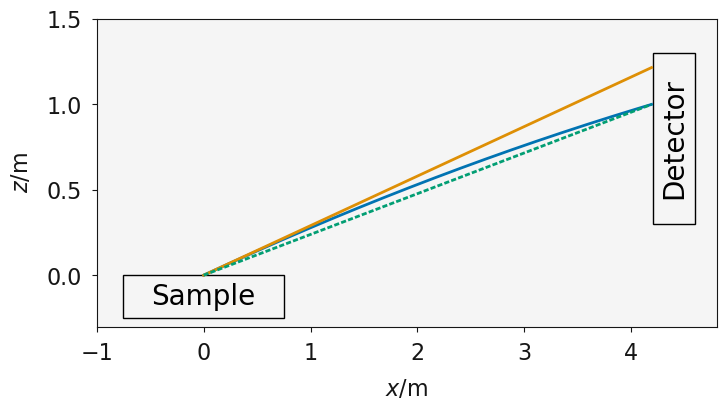 The effect of gravity for a neutron with a velocity of 20 ms-1; the solid blue line shows the trajectory of a neutron reflected from a surface under the influence of gravity, the dashed green line shows the trajectory without gravity if no correction, the solid orange line shows the true trajectory if the reflection were to occur with no gravity present.
The figure above shows the trajectory of a neutron reflecting from a sample and being detected on the detector (the blue line). Initially assuming that all of the neutrons are incident at the point \((0, 0)\) (the influence of beam and sample width is considered below). During the trajectory, the neutron is acted on by the force of gravity, leading to the parabolic motion shown. It is clear that if \(\theta\) were calculated without accounting for gravity (dashed green line), then the angle would be underestimated.
The trajectory for the detected neutron can be found by considering the kinematic equations of motion. The time taken for the neutron to travel from \(x=x_0\) to \(x=x_d\) is,
where, \(v_x\) is the velocity of the neutron in the x-dimension. It is assumed that the velocity in this dimension is the main component of the total velocity and that this doesn’t change over time. Therefore, we can calculate \(v_x\) from the neutron’s wavelength as,
This can be found as follows.
[16]:
data.events.coords["velocity"] = sc.to_unit(HDM / data.events.coords['wavelength'], 'm/s')
data.events.coords["velocity"]
[16]:
- (event: 259478)float64m/s638.3, 295.66, ..., 898.98, 751.92
Values:
array([638.29571175, 295.65903565, 734.15724132, ..., 892.7682167 ,
       898.9826174 , 751.91996421])
It is assumed that the parabolic motion does not reach a maximum before the neutron is incident on the detector. Therefore, the velocity in the \(y\)-dimension at the time of reflection can be found,
where \(z_0\) is the initial position of the neutron, \(z_0 = 0\), and \(a\) is the acceleration due to gravity, \(a = -g = 9.80665\;\text{ms}^{-2}\). Using this, the \(z\)-position of the neutron can be found at any time, \(t\),
or any \(x\)-position (with \(v_z(0)\) expanded),
The derivative of this with respect to \(x\) can then be found,
This can be simplified when \(x=x_0\) to,
From which \(\theta\) can be found,
where, \(\omega\) is the angle of the sample relative to the laboratory horizon.
We can show this in action, first by defining a function for the derivative above.
[17]:
def z_dash0(velocity, x_origin, z_origin, x_measured, z_measured):
    """
    Evaluation of the first dervative of the kinematic equations
    for for the trajectory of a neutron reflected from a surface.

    :param velocity: Neutron velocity
    :type velocity: scipp._scipp.core.VariableView
    :param x_origin: The z-origin position for the reflected neutron
    :type x_origin: scipp._scipp.core.Variable
    :param z_origin: The y-origin position for the reflected neutron
    :type z_origin: scipp._scipp.core.Variable
    :param x_measured: The z-measured position for the reflected neutron
    :type x_measured: scipp._scipp.core.Variable
    :param z_measured: The y-measured position for the reflected neutron
    :type z_measured: scipp._scipp.core.Variable

    :return: The gradient of the trajectory of the neutron at the origin position.
    :rtype: scipp._scipp.core.VariableView
    """
    velocity2 = velocity * velocity
    x_diff = x_measured - x_origin
    z_diff = z_measured - z_origin
    return -0.5 * sc.norm(G_ACC) * x_diff / velocity2 + z_diff / x_diff
The angle is found by evaluating the position of each pixel with respect to the sample position.
[18]:
z_measured = data.coords['position'].fields.z
x_measured = data.coords['position'].fields.x
z_origin = data.coords['sample_position'].fields.z
x_origin = data.coords['sample_position'].fields.x
The gradient and hence the angle can then be found.
[19]:
z_dash = z_dash0(
    data.bins.coords["velocity"],
    x_origin,
    z_origin,
    x_measured,
    z_measured)
intercept = z_origin - z_dash * x_origin
z_true = x_measured * z_dash + intercept
angle = sc.to_unit(
    sc.atan(z_true / x_measured).bins.constituents["data"],
    'deg')
angle
[19]:
- (event: 259478)float64deg1.31, 1.3, ..., 0.58, 0.58
Values:
array([1.31041603, 1.30000491, 1.31111022, ..., 0.57779029, 0.57780971,
       0.5772127 ])
The value of \(\theta\) can then be found by accounting for the sample angle, \(\omega\).
[20]:
omega = 0.0 * sc.units.deg
data.events.coords['theta'] = -omega + angle
[21]:
data
[21]:
- detector_id: 9216
- wavelength: 1
- detector_id(detector_id)int321, 2, ..., 9215, 9216
Values:
array([ 1, 2, 3, ..., 9214, 9215, 9216], dtype=int32) - position(detector_id)vector_3_float64m[ 4.12644383 -0.064 0.09459759], [ 4.12644383 -0.05987097 0.09459759], ..., [4. 0.05987097 0. ], [4. 0.064 0. ]
Values:
array([[ 4.12644383, -0.064 , 0.09459759], [ 4.12644383, -0.05987097, 0.09459759], [ 4.12644383, -0.05574194, 0.09459759], ..., [ 4. , 0.05574194, 0. ], [ 4. , 0.05987097, 0. ], [ 4. , 0.064 , 0. ]]) - sample_position()vector_3_float64m[0. 0. 0.]
Values:
array([0., 0., 0.]) - source_position()vector_3_float64m[-15. 0. 0.]
Values:
array([-15., 0., 0.]) - wavelength(wavelength [bin-edge])float64Å2.4, 15.0
Values:
array([ 2.4, 15. ])
- (detector_id, wavelength)DataArrayViewbinned data [len=0, len=0, ..., len=0, len=0]
Values:
[<scipp.DataArray>
Dimensions: Sizes[event:0, ]
Coordinates:
  pulse_time              datetime64             [ns]  (event)  []
  theta                     float64            [deg]  (event)  []
  velocity                  float64            [m/s]  (event)  []
  wavelength                float64             [Å]  (event)  []
Data:
                            float32         [counts]  (event)  []  []

, <scipp.DataArray>
Dimensions: Sizes[event:0, ]
Coordinates:
  pulse_time              datetime64             [ns]  (event)  []
  theta                     float64            [deg]  (event)  []
  velocity                  float64            [m/s]  (event)  []
  wavelength                float64             [Å]  (event)  []
Data:
                            float32         [counts]  (event)  []  []

, ..., <scipp.DataArray>
Dimensions: Sizes[event:0, ]
Coordinates:
  pulse_time              datetime64             [ns]  (event)  []
  theta                     float64            [deg]  (event)  []
  velocity                  float64            [m/s]  (event)  []
  wavelength                float64             [Å]  (event)  []
Data:
                            float32         [counts]  (event)  []  []

, <scipp.DataArray>
Dimensions: Sizes[event:0, ]
Coordinates:
  pulse_time              datetime64             [ns]  (event)  []
  theta                     float64            [deg]  (event)  []
  velocity                  float64            [m/s]  (event)  []
  wavelength                float64             [Å]  (event)  []
Data:
                            float32         [counts]  (event)  []  []

]
- experiment_title()stringcommissioning
Values:
'commissioning' - instrument_name()stringAMOR
Values:
'AMOR' - start_time()string2020-11-25T16:03:10.000000000
Values:
'2020-11-25T16:03:10.000000000'
This can be visualised like the wavelength and time-of-flight data earlier, or as a two-dimensional histogram of the intensity as a function of \(\lambda\)/\(\theta\).
[22]:
max_t = sc.max(data.events.coords['theta'])
min_t = sc.min(data.events.coords['theta'])
bins_t = sc.linspace(
    dim='theta',
    start=min_t.value,
    stop=max_t.value,
    num=50,
    unit=data.events.coords['theta'].unit)
max_w = sc.max(wavelength_range)
min_w = sc.min(wavelength_range)
bins = sc.linspace(
    dim='wavelength',
    start=min_w.value,
    stop=max_w.value,
    num=100,
    unit=data.events.coords['wavelength'].unit)
sc.bin(data.events, edges=[bins_t, bins]).bins.sum().plot()
Determination of \(q_z\)-vector
The \(\lambda\) and \(\theta\) can be brought together to calculate the the wavevector, \(q_z\),
This is shown below.
[23]:
data.events.coords['qz'] = 4. * np.pi * sc.sin(
    data.events.coords['theta']) / data.events.coords['wavelength']
[24]:
data.events
[24]:
- event: 259478
- pulse_time(event)datetime64ns2020-11-25T15:04:39.000000000, 2020-11-25T15:03:23.000000000, ..., 2020-11-25T15:03:38.000000000, 2020-11-25T15:05:09.000000000
Values:
array(['2020-11-25T15:04:39.000000000', '2020-11-25T15:03:23.000000000', '2020-11-25T15:04:29.000000000', ..., '2020-11-25T15:03:20.000000000', '2020-11-25T15:03:38.000000000', '2020-11-25T15:05:09.000000000'], dtype='datetime64[ns]') - qz(event)float641/Å0.05, 0.02, ..., 0.03, 0.02
Values:
array([0.04636823, 0.02130719, 0.05336022, ..., 0.02859755, 0.02879758, 0.02406176]) - theta(event)float64deg1.31, 1.3, ..., 0.58, 0.58
Values:
array([1.31041603, 1.30000491, 1.31111022, ..., 0.57779029, 0.57780971, 0.5772127 ]) - velocity(event)float64m/s638.3, 295.66, ..., 898.98, 751.92
Values:
array([638.29571175, 295.65903565, 734.15724132, ..., 892.7682167 , 898.9826174 , 751.91996421]) - wavelength(event)float64Å6.2, 13.38, ..., 4.4, 5.26
Values:
array([ 6.1978076 , 13.38039273,  5.38853775, ...,  4.43119943,
        4.40056786,  5.26124348])
- (event)float32counts1.0, 1.0, ..., 1.0, 1.0σ = 1.0, 1.0, ..., 1.0, 1.0
Values:
array([1., 1., 1., ..., 1., 1., 1.], dtype=float32)

Variances (σ²):
array([1., 1., 1., ..., 1., 1., 1.], dtype=float32)
We can then investigate the intensity as a function of \(q_z\).
[25]:
max_q = 0.08 * sc.Unit('1/angstrom')
min_q = 0.008 * sc.Unit('1/angstrom')
bins_q = sc.Variable(
    values=np.linspace(min_q.value, max_q.value, 200),
    unit=data.events.coords['qz'].unit,
    dims=['qz'])
sc.histogram(data.events, bins=bins_q).plot(norm='log')
Illumination correction
The above intensity as a function of \(q_z\) fails to account for the difference in illumination as a function of \(\theta\), due to the size of the beam which illuminates the sample decreases with increasing \(\theta\).
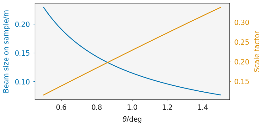 The effect of \(\theta\) on the beam size on the sample (blue line) and the resulting scale factor where the size of the sample is considered (orange line); where the beam size is 2 mm and the sample is 10 mm.
Using the assumption that the beam size describes the full width at half maximum of the beam, the following function can be used to determine the scale factor necessary to account for the illumination variation as a function of \(\theta\).
[26]:
def illumination_correction(beam_size, sample_size, theta):
    """
    The factor by which the intensity should be multiplied to account for the
    scattering geometry, where the beam is Gaussian in shape.

    :param: beam_size: Width of incident beam
    :type beam_size: scipp._scipp.core.Variable
    :param sample_size: Width of sample in the dimension of the beam
    :type sample_size: scipp._scipp.core.Variable
    :param theta: Incident angle
    :type theta: scipp._scipp.core.Variable

    :return: Correction factor
    :rtype: scipp._scipp.core.Variable
    """
    beam_on_sample = beam_size / sc.sin(theta)
    fwhm_to_std = 2 * np.sqrt(2 * np.log(2))
    scale_factor = erf(
        (sample_size / beam_on_sample * fwhm_to_std).values)
    return sc.Variable(values=scale_factor, dims=theta.dims)
This illumination correction scale factor is applied to each event as follows.
[27]:
data.events.data /= illumination_correction(
    2 * sc.Unit('mm'),
    10 * sc.Unit('mm'),
    data.events.coords['theta'])
[28]:
data.events.data
[28]:
- (event: 259478)float32counts3.37, 3.4, ..., 7.5, 7.51σ = 3.37, 3.4, ..., 7.5, 7.51
Values:
array([3.3710356, 3.3967533, 3.3693357, ..., 7.4991827, 7.498933 ,
       7.506616 ], dtype=float32)

Variances (σ²):
array([11.36388 , 11.537933, 11.352423, ..., 56.23774 , 56.233994,
       56.349285], dtype=float32)
We can then show the reflected intensity as a function of a linear \(q_z\) as shown below.
[29]:
max_q = 0.08 * sc.Unit('1/angstrom')
min_q = 0.008 * sc.Unit('1/angstrom')
bins_q = sc.linspace(
    dim='qz',
    start=min_q.value,
    stop=max_q.value,
    num=200,
    unit=data.events.coords['qz'].unit)
sc.histogram(data.events, bins=bins_q).plot(norm='log')
Resolution functions
We will consider three contributions to the resolution function at the Amor instrument:
\(\sigma \lambda/\lambda\): this is due to the double-blind chopper and depends on the distance between the two choppers, \(d_{CC}\), and the distance from the halfway between the two choppers to the detector \(d_{CD}\),
[30]:
chopper_chopper_distance=0.49 * sc.units.m
data.attrs["sigma_lambda_by_lambda"] = chopper_chopper_distance / (
    data.coords["position"].fields.z - data.coords["source_position"].fields.z)
data.attrs["sigma_lambda_by_lambda"] /= 2 * np.sqrt(2 * np.log(2))
\(\sigma \gamma/\theta\): this is to account for the spatial resolution of the detector pixels, which have a FWHM of \(\Delta z \approx 0.5\;\text{mm}\) and the sample to detector distance, \(d_{SD}\),
[31]:
spatial_resolution = 0.0005 * sc.units.m
fwhm = sc.to_unit(
    sc.atan(
        spatial_resolution / (
                data.coords["position"].fields.z -
                data.coords["source_position"].fields.z)),"deg",)
sigma_gamma = fwhm / (2 * np.sqrt(2 * np.log(2)))
data.attrs["sigma_gamma_by_theta"] = sigma_gamma / data.bins.coords['theta']
\(\sigma \theta/\theta\): finally, this accounts for the width of the beam on the sample or the size of the sample (which ever is smaller), the FWHM is the range of possible \(\theta\)-values, accounting for the gravity correction discussed above and the sample/beam geometry,
[32]:
beam_size = 0.001 * sc.units.m
sample_size = 0.5 * sc.units.m
beam_on_sample = beam_size / sc.sin(data.bins.coords['theta'])
half_beam_on_sample = (beam_on_sample / 2.0)
offset_positive = data.coords['sample_position'].copy()
offset_positive.fields.x + half_beam_on_sample
offset_negative = data.coords['sample_position'].copy()
offset_negative.fields.x - half_beam_on_sample
z_measured = data.coords["position"].fields.z
x_measured = data.coords["position"].fields.x
x_origin = offset_positive.fields.x
z_origin = offset_positive.fields.z
z_dash = z_dash0(data.bins.coords["velocity"], x_origin, z_origin, x_measured, z_measured)
intercept = z_origin - z_dash * x_origin
z_true = x_measured * z_dash + intercept
angle_max = sc.to_unit(sc.atan(z_true / x_measured), 'deg')
x_origin = offset_negative.fields.x
z_origin = offset_negative.fields.z
z_dash = z_dash0(data.bins.coords["velocity"], x_origin, z_origin, x_measured, z_measured)
intercept = z_origin - z_dash * x_origin
z_true = x_measured * z_dash + intercept
angle_min = sc.to_unit(sc.atan(z_true / x_measured), 'deg')
fwhm_to_std = 2 * np.sqrt(2 * np.log(2))
sigma_theta_position = (angle_max - angle_min) / fwhm_to_std
data.attrs["sigma_theta_by_theta"] = sigma_theta_position / data.bins.coords['theta']
These three contributors to the resolution function are combined to give the total resolution function,
[33]:
data.events.attrs['sigma_q_by_q'] = sc.sqrt(
    data.attrs['sigma_lambda_by_lambda'] * data.attrs['sigma_lambda_by_lambda']
    + data.attrs['sigma_gamma_by_theta'] * data.attrs['sigma_gamma_by_theta']
    + data.attrs["sigma_theta_by_theta"] * data.attrs["sigma_theta_by_theta"]).bins.constituents['data']
Normalisation
The above steps are performed both on the sample of interest and a reference supermirror, using the AmorData class, thus enabling normalisation to be achieved.
[34]:
sample = AmorData(data_file)
reference = AmorData(reference_file)
/usr/share/miniconda/envs/tempenv/lib/python3.7/scippneutron/file_loading/_log_data.py:23: UserWarning: Skipped loading /entry/stages/com due to:
NXlog 'com' has time and value datasets of different shapes
  warn(f"Skipped loading {group.path} due to:\n{e}")
/usr/share/miniconda/envs/tempenv/lib/python3.7/scippneutron/file_loading/_log_data.py:23: UserWarning: Skipped loading /entry/stages/coz due to:
NXlog 'coz' has time and value datasets of different shapes
  warn(f"Skipped loading {group.path} due to:\n{e}")
/usr/share/miniconda/envs/tempenv/lib/python3.7/scippneutron/file_loading/_log_data.py:23: UserWarning: Skipped loading /entry/stages/diaphragms/middle focus/slot due to:
NXlog 'slot' has an empty value dataset
  warn(f"Skipped loading {group.path} due to:\n{e}")
/usr/share/miniconda/envs/tempenv/lib/python3.7/scippneutron/file_loading/_log_data.py:23: UserWarning: Skipped loading /entry/stages/diaphragms/virtual source/horizontal due to:
NXlog 'horizontal' has an empty value dataset
  warn(f"Skipped loading {group.path} due to:\n{e}")
/usr/share/miniconda/envs/tempenv/lib/python3.7/scippneutron/file_loading/_log_data.py:23: UserWarning: Skipped loading /entry/stages/diaphragms/virtual source/vertical due to:
NXlog 'vertical' has an empty value dataset
  warn(f"Skipped loading {group.path} due to:\n{e}")
/usr/share/miniconda/envs/tempenv/lib/python3.7/scippneutron/file_loading/_log_data.py:23: UserWarning: Skipped loading /entry/stages/som due to:
NXlog 'som' has time and value datasets of different shapes
  warn(f"Skipped loading {group.path} due to:\n{e}")
/usr/share/miniconda/envs/tempenv/lib/python3.7/scippneutron/file_loading/_log_data.py:23: UserWarning: Skipped loading /entry/stages/soz due to:
NXlog 'soz' has time and value datasets of different shapes
  warn(f"Skipped loading {group.path} due to:\n{e}")
These result in the plots shown below.
[35]:
sc.histogram(sample.data.events, bins=bins_q).plot(norm='log')
[36]:
sc.histogram(reference.data.events, bins=bins_q).plot(norm='log')
The specification of the supermirror defines the normalisation that is used for it.
[37]:
m_value = 5
supermirror_critical_edge = (0.022) * sc.Unit('1/angstrom')
supermirror_max_q = m_value * supermirror_critical_edge
supermirror_alpha = 0.25 / 0.088 * sc.units.angstrom
normalisation = sc.ones(
    dims=['event'],
    shape=reference.data.events.data.shape)
The data array is first masked at values greater than the upper limit of the supermirror.
[38]:
reference.data.events.masks['normalisation'] = reference.data.events.coords['qz'] >= supermirror_max_q
The value of the \(q\)-dependent normalisation, \(n(q)\), is then defined as such that \(n(q)=1\) for values of \(q\) less then the critical edge of the supermirror and for values between this and the supermirror maximum the normalisation is,
[39]:
lim = (reference.data.events.coords['qz'] < supermirror_critical_edge).astype(sc.dtype.float32)
[40]:
nq = 1.0 / (1.0 - supermirror_alpha * (reference.data.events.coords['qz'] - supermirror_critical_edge))
[41]:
normalisation = lim + (1 - lim) * nq
Applying this normalisation to the reference measurement data will return the neutron intensity as a function of \(q\).
[42]:
reference.data.bins.constituents['data'].data = reference.data.events.data / normalisation.astype(sc.dtype.float32)
[43]:
sc.histogram(reference.data.events, bins=bins_q).plot(norm='log')
Binning this normalised description on the neutron intensity and the sample measurement in the same \(q\)-values allows the normalisation to be applied to the sample (note that scaling between these to measurements to account for counting time may be necessary).
[44]:
binned_sample = sc.histogram(sample.data.events, bins=bins_q)
binned_reference = sc.histogram(reference.data.events, bins=bins_q)
[45]:
normalised_sample = binned_sample / binned_reference
[46]:
normalised_sample.plot(norm='log')