Direct beam iterations for LoKI#
Introduction#
This notebook is used to compute the direct beam function for the LoKI detectors. It uses data recorded during the detector test at the Larmor instrument.
Description of the procedure:
The idea behind the direct beam iterations is to determine an efficiency of the detectors as a function of wavelength. To calculate this, it is possible to compute \(I(Q)\) for the full wavelength range, and for individual slices (bands) of the wavelength range. If the direct beam function used in the \(I(Q)\) computation is correct, then \(I(Q)\) curves for the full wavelength range and inside the bands should overlap.
In the following notebook, we will:
Create a workflow to compute \(I(Q)\) inside a set of wavelength bands (the number of wavelength bands will be the number of data points in the final direct beam function)
Create a flat direct beam function, as a function of wavelength, with wavelength bins corresponding to the wavelength bands
Calculate inside each band by how much one would have to multiply the final \(I(Q)\) so that the curve would overlap with the full-range curve (we compute the full-range data by making a copy of the workflow but setting only a single wavelength band that contains all wavelengths)
Multiply the direct beam values inside each wavelength band by this factor
Compare the full-range \(I(Q)\) to a theoretical reference and add the corresponding additional scaling to the direct beam function
Iterate until the changes to the direct beam function become small
[1]:
import scipp as sc
import plopp as pp
from ess import sans
from ess import loki
import ess.loki.data  # noqa: F401
from ess.sans.types import *
Create and configure the workflow#
We begin by creating the Loki workflow object (this is a sciline.Pipeline which can be consulted for advanced usage). The files we use here come from a Loki detector test at Larmor, so we use the corresponding workflow:
[2]:
workflow = loki.LokiAtLarmorWorkflow()
We configure the workflow be defining the series of masks filenames and bank names to reduce. In this case there is just a single bank:
[3]:
workflow = sans.with_pixel_mask_filenames(
    workflow, masks=loki.data.loki_tutorial_mask_filenames()
)
workflow[NeXusDetectorName] = 'larmor_detector'
Downloading file 'mask_new_July2022.xml' from 'https://public.esss.dk/groups/scipp/ess/loki/2/mask_new_July2022.xml' to '/home/runner/.cache/ess/loki'.
The workflow can be visualized as a graph. For readability we show only sub-workflow for computing IofQ[Sample]. The workflow can actually compute the full BackgroundSubtractedIofQ, which applies and equivalent workflow to the background run, before a subtraction step:
[4]:
workflow.visualize(IntensityQ[SampleRun], compact=True, graph_attr={'rankdir': 'LR'})
[4]:

Note the red boxes which indicate missing input parameters. We can set these missing parameters, as well as parameters where we do not want to use the defaults:
[5]:
# Wavelength binning parameters
wavelength_min = sc.scalar(1.0, unit='angstrom')
wavelength_max = sc.scalar(13.0, unit='angstrom')
n_wavelength_bins = 50
n_wavelength_bands = 50

workflow[WavelengthBins] = sc.linspace(
    'wavelength', wavelength_min, wavelength_max, n_wavelength_bins + 1
)
workflow[WavelengthBands] = sc.linspace(
    'wavelength', wavelength_min, wavelength_max, n_wavelength_bands + 1
)


workflow[CorrectForGravity] = True
workflow[UncertaintyBroadcastMode] = UncertaintyBroadcastMode.upper_bound
workflow[ReturnEvents] = False

workflow[QBins] = sc.linspace(dim='Q', start=0.01, stop=0.3, num=101, unit='1/angstrom')
Configuring data to load#
We have not configured which files we want to load. In this tutorial, we use helpers to fetch the tutorial data which return the filenames of the cached files. In a real use case, you would set these parameters manually:
[6]:
workflow[Filename[SampleRun]] = loki.data.loki_tutorial_sample_run_60339()
workflow[Filename[BackgroundRun]] = loki.data.loki_tutorial_background_run_60393()
workflow[Filename[TransmissionRun[SampleRun]]] = (
    loki.data.loki_tutorial_sample_transmission_run()
)
workflow[Filename[TransmissionRun[BackgroundRun]]] = loki.data.loki_tutorial_run_60392()
workflow[Filename[EmptyBeamRun]] = loki.data.loki_tutorial_run_60392()
Downloading file '60339-2022-02-28_2215.nxs' from 'https://public.esss.dk/groups/scipp/ess/loki/2/60339-2022-02-28_2215.nxs' to '/home/runner/.cache/ess/loki'.
Downloading file '60393-2022-02-28_2215.nxs' from 'https://public.esss.dk/groups/scipp/ess/loki/2/60393-2022-02-28_2215.nxs' to '/home/runner/.cache/ess/loki'.
Downloading file '60394-2022-02-28_2215.nxs' from 'https://public.esss.dk/groups/scipp/ess/loki/2/60394-2022-02-28_2215.nxs' to '/home/runner/.cache/ess/loki'.
Downloading file '60392-2022-02-28_2215.nxs' from 'https://public.esss.dk/groups/scipp/ess/loki/2/60392-2022-02-28_2215.nxs' to '/home/runner/.cache/ess/loki'.
Finding the beam center#
Looking carefully at the workflow above, one will notice that there is a missing parameter from the workflow: the red box that contains the BeamCenter type. Before we can proceed with computing the direct beam function, we therefore have to first determine the center of the beam.
There are more details on how this is done in the beam center finder notebook, but for now we simply reuse the workflow (by making a copy), and inserting the provider that will compute the beam center.
For now, we compute the beam center only for the rear detector (named ‘larmor_detector’) but apply it to all banks (currently there is only one bank). The beam center may need to be computed or applied differently to each bank, see scipp/esssans#28. We use a center-of-mass approach to find the beam center:
[7]:
center = sans.beam_center_from_center_of_mass(workflow)
center
[7]:
- ()vector3m[-0.02914868 -0.01816138 0. ]
Values:
array([-0.02914868, -0.01816138,  0.        ])
and set that value in our workflow
[8]:
workflow[BeamCenter] = center
Expected intensity at zero Q#
The sample used in the experiment has a known \(I(Q)\) profile, and we need it to calibrate the absolute intensity of our \(I(Q)\) results (relative differences between wavelength band and full-range results are not sufficient).
We load this theoretical reference curve, and compute the \(I_{0}\) intensity at the lower \(Q\) bound of the range covered by the instrument.
[9]:
from scipp.scipy.interpolate import interp1d

Iq_theory = sc.io.load_hdf5(loki.data.loki_tutorial_poly_gauss_I0())
f = interp1d(Iq_theory, 'Q')
I0 = f(sc.midpoints(workflow.compute(QBins))).data[0]
I0
Downloading file 'PolyGauss_I0-50_Rg-60.h5' from 'https://public.esss.dk/groups/scipp/ess/loki/2/PolyGauss_I0-50_Rg-60.h5' to '/home/runner/.cache/ess/loki'.
[9]:
- ()float64𝟙43.19421720556363
Values:
array(43.19421721)
A single direct beam function for all layers#
As a first pass, we compute a single direct beam function for all the detector pixels combined.
We compute the \(I(Q)\) inside the wavelength bands and the full wavelength range, derive a direct beam factor per wavelength band, and also add absolute scaling using the reference \(I_{0}\) value
[10]:
results = sans.direct_beam(workflow=workflow, I0=I0, niter=6)
# Unpack the final result
iofq_full = results[-1]['iofq_full']
iofq_bands = results[-1]['iofq_bands']
direct_beam_function = results[-1]['direct_beam']
We now compare the \(I(Q)\) curves in each wavelength band to the one for the full wavelength range (black).
[11]:
pp.plot(
    {**sc.collapse(iofq_bands, keep='Q'), **{'full': iofq_full}},
    norm='log',
    color={'full': 'k'},
    legend=False,
)
[11]:

The overlap is satisfactory, and we can now inspect the direct beam function we have computed:
[12]:
direct_beam_function.plot(vmax=1)
[12]:

Finally, as a sanity check, we compare our final \(I(Q)\) for the full wavelength range to the theoretical reference:
[13]:
pp.plot(
    {'reference': Iq_theory, 'data': iofq_full},
    color={'reference': 'darkgrey', 'data': 'C0'},
    norm='log',
)
[13]:

Direct beam function per layer#
The LoKI detector tubes are arranged in layers along the beam path, where the layers closest to the sample will receive most of the scattered neutrons, while occulting the layers behind them.
A refinement to the above procedure is to compute a direct beam function for each layer of tubes individually. We also use the 4 thick layers of tubes, but in principle, this could also be done for 28 different layers (made from the layer and straw dimensions) if a run with enough events is provided (or many runs are combined together).
The only other difference compared to the computation above is that we now want our final result to preserve the 'layer' dimension, so that the dimensions of our result are ['layer', 'Q'].
[14]:
workflow[DimsToKeep] = ['layer']
Now we are able to run the direct-beam iterations on a per-layer basis:
[15]:
results_layers = sans.direct_beam(workflow=workflow, I0=I0, niter=6)
# Unpack the final result
iofq_full_layers = results_layers[-1]['iofq_full']
iofq_bands_layers = results_layers[-1]['iofq_bands']
direct_beam_function_layers = results_layers[-1]['direct_beam']
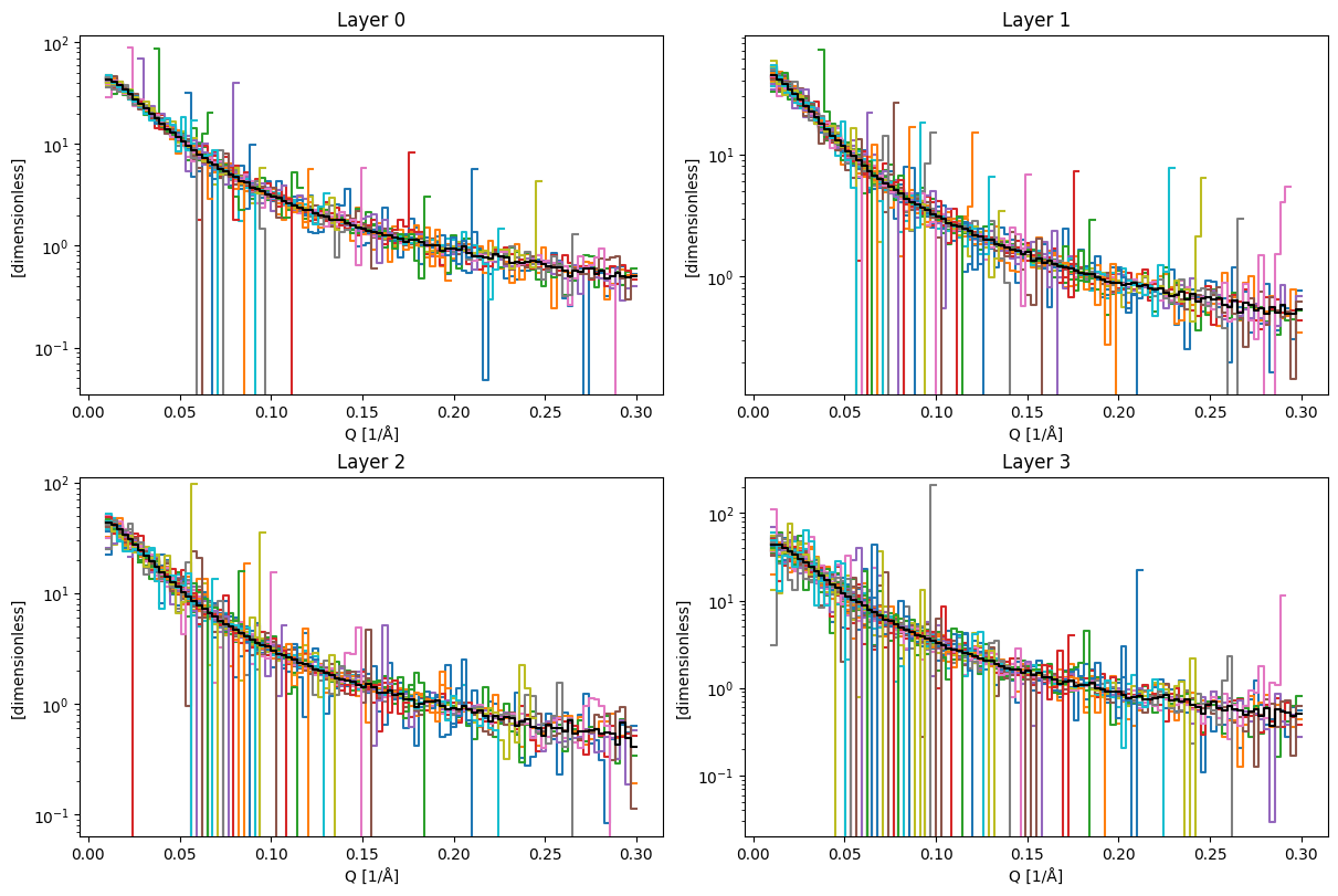
We can now inspect the wavelength slices for the 4 layers.
[16]:
plots = [
    pp.plot(
        {
            **sc.collapse(iofq_bands_layers['layer', i], keep='Q'),
            **{'full': iofq_full_layers['layer', i]},
        },
        norm='log',
        color={'full': 'k'},
        legend=False,
        title=f'Layer {i}',
    )
    for i in range(4)
]

(plots[0] + plots[1]) / (plots[2] + plots[3])
[16]:
Now the direct beam function inside each layer looks like:
[17]:
pp.plot(sc.collapse(direct_beam_function_layers, keep='wavelength'))
[17]:

And finally, for completeness, we compare the \(I(Q)\) to the theoretical reference inside each layer.
[18]:
layers = sc.collapse(iofq_full_layers, keep='Q')
pp.plot(
    {**{'reference': Iq_theory}, **layers},
    color={
        **{'reference': 'darkgrey'},
        **{key: f'C{i}' for i, key in enumerate(layers)},
    },
    norm='log',
)
[18]:

Combining multiple runs to boost signal#
It is common practise to combine the events from multiple runs to improve the statistics on the computed \(I(Q)\), and thus obtain a more robust direct beam function.
To achieve this, we need to replace the SampleRun and BackgroundRun file names with parameter series. We then need to supply additional providers which will merge the events from the runs appropriately (note that these providers will merge both the detector and the monitor events).
We first define a list of file names for the sample and background runs (two files for each):
[19]:
sample_runs = [
    loki.data.loki_tutorial_sample_run_60250(),
    loki.data.loki_tutorial_sample_run_60339(),
]
background_runs = [
    loki.data.loki_tutorial_background_run_60248(),
    loki.data.loki_tutorial_background_run_60393(),
]
Downloading file '60250-2022-02-28_2215.nxs' from 'https://public.esss.dk/groups/scipp/ess/loki/2/60250-2022-02-28_2215.nxs' to '/home/runner/.cache/ess/loki'.
Downloading file '60248-2022-02-28_2215.nxs' from 'https://public.esss.dk/groups/scipp/ess/loki/2/60248-2022-02-28_2215.nxs' to '/home/runner/.cache/ess/loki'.
We modify the workflow, setting multiple background and sample runs:
[20]:
# Reset workflow
workflow[DimsToKeep] = []

# Transform base workflow to use multiple sample and background runs
workflow = sans.with_background_runs(workflow, runs=background_runs)
workflow = sans.with_sample_runs(workflow, runs=sample_runs)
If we now visualize the workflow, we can see that every step for the SampleRun and BackgroundRun branches are now replicated (drawn as 3D-looking boxes instead of flat rectangles, set compact=False to show flattened version). There is also the new merge_contributions step that combines the events from the two runs, just before the normalization.
[21]:
workflow.visualize(BackgroundSubtractedIofQ, compact=True, graph_attr={'rankdir': 'LR'})
[21]:

We run the direct beam iterations again and compare with our original results.
[22]:
results = sans.direct_beam(workflow=workflow, I0=I0, niter=6)
# Unpack the final result
iofq_full_new = results[-1]['iofq_full']
iofq_bands_new = results[-1]['iofq_bands']
direct_beam_function_new = results[-1]['direct_beam']
[23]:
pp.plot({'one run': direct_beam_function, 'two runs': direct_beam_function_new})
[23]:

[24]:
pp.plot(
    {'reference': Iq_theory, 'one run': iofq_full, 'two runs': iofq_full_new},
    color={'reference': 'darkgrey', 'one run': 'C0', 'two runs': 'C1'},
    norm='log',
)
[24]:
