Scaling#
MTZ IO#
ess.nmx has MTZ IO helper functions. They can be used as providers in a workflow of scaling routine.
They are wrapping MTZ IO functions of gemmi.
[1]:
%matplotlib inline
[2]:
import gemmi
from ess.nmx.mtz_io import (
    read_mtz_file,
    mtz_to_pandas,
    MTZFilePath,
    get_unique_space_group,
    MtzDataFrame,
    merge_mtz_dataframes,
)
from ess.nmx.data import get_small_random_mtz_samples


small_mtz_sample = get_small_random_mtz_samples()[0]
mtz = read_mtz_file(MTZFilePath(small_mtz_sample))
df = mtz_to_pandas(mtz)
df.head()
Downloading file 'mtz_random_samples.tar.gz' from 'https://public.esss.dk/groups/scipp/ess/nmx/mtz_random_samples.tar.gz' to '/home/runner/.cache/essnmx/0'.
Untarring contents of '/home/runner/.cache/essnmx/0/mtz_random_samples.tar.gz' to '/home/runner/.cache/essnmx/0/mtz_random_samples.tar.gz.untar'
[2]:
| I | SIGI | LAMBDA | H | K | L | |
|---|---|---|---|---|---|---|
| 0 | 130.737228 | 16.514244 | 3.199999 | -65.0 | 34.0 | 94.0 |
| 1 | 127.729103 | 13.795578 | 3.199982 | 30.0 | -8.0 | -43.0 |
| 2 | 121.405731 | 16.670300 | 3.199974 | 78.0 | 91.0 | 81.0 |
| 3 | 119.699654 | 12.158858 | 3.199864 | -25.0 | 20.0 | -75.0 |
| 4 | 116.459991 | 16.823048 | 3.199790 | 18.0 | -98.0 | 69.0 |
Build Pipeline#
Scaling routine includes: - Reducing individual MTZ dataset - Merging MTZ dataset - Reducing merged MTZ dataset
These operations are done on pandas dataframe as recommended in gemmi. And multiple MTZ files are expected, so we need to use sciline.ParamTable.
[3]:
import pandas as pd
import sciline as sl
import scipp as sc

from ess.nmx.mtz_io import providers as mtz_io_providers, default_parameters as mtz_io_params
from ess.nmx.mtz_io import SpaceGroupDesc
from ess.nmx.scaling import providers as scaling_providers, default_parameters as scaling_params
from ess.nmx.scaling import (
    WavelengthBins,
    FilteredEstimatedScaledIntensities,
    ReferenceWavelength,
    ScaledIntensityLeftTailThreshold,
    ScaledIntensityRightTailThreshold,
)

pl = sl.Pipeline(
    providers=mtz_io_providers + scaling_providers,
    params={
        SpaceGroupDesc: "C 1 2 1",
        ReferenceWavelength: sc.scalar(
            3, unit=sc.units.angstrom
        ),  # Remove it if you want to use the middle of the bin
        ScaledIntensityLeftTailThreshold: sc.scalar(
            0.1,  # Increase it to remove more outliers
        ),
        ScaledIntensityRightTailThreshold: sc.scalar(
            4.0,  # Decrease it to remove more outliers
        ),
        **mtz_io_params,
        **scaling_params,
        WavelengthBins: 250,
    },
)
pl
[3]:
| Name | Value | Source |
|---|---|---|
| EstimatedScaleFactor |
estimate_scale_factor_per_hkl_asu_from_referenceess.nmx.scaling.estimate_scale_factor_per_hkl_asu_from_reference | |
| EstimatedScaledIntensities |
average_roughly_scaled_intensitiesess.nmx.scaling.average_roughly_scaled_intensities | |
| FilteredEstimatedScaledIntensities |
cut_tailsess.nmx.scaling.cut_tails | |
| FittingResult |
fit_wavelength_scale_factor_polynomialess.nmx.scaling.fit_wavelength_scale_factor_polynomial | |
| IntensityColumnName | I | |
| MTZFilePath | ||
| Mtz |
read_mtz_fileess.nmx.mtz_io.read_mtz_file | |
| MtzDataFrame |
process_single_mtz_to_dataframeess.nmx.mtz_io.process_single_mtz_to_dataframe | |
| NMXMtzDataArray |
nmx_mtz_dataframe_to_scipp_dataarrayess.nmx.mtz_io.nmx_mtz_dataframe_to_scipp_dataarray | |
| NMXMtzDataFrame |
process_mtz_dataframeess.nmx.mtz_io.process_mtz_dataframe | |
| ReciprocalAsu |
get_reciprocal_asuess.nmx.mtz_io.get_reciprocal_asu | |
| ReferenceIntensities |
get_reference_intensitiesess.nmx.scaling.get_reference_intensities | |
| ReferenceWavelength |
<scipp.Variable> () ...<scipp.Variable> () int64 [Å] 3 |
|
| ScaledIntensityLeftTailThreshold |
<scipp.Variable> () f...<scipp.Variable> () float64 [dimensionless] 0.1 |
|
| ScaledIntensityRightTailThreshold |
<scipp.Variable> () f...<scipp.Variable> () float64 [dimensionless] 2 |
|
| SelectedReferenceWavelength |
get_reference_wavelengthess.nmx.scaling.get_reference_wavelength | |
| SpaceGroup | ||
| SpaceGroup | NoneType |
get_space_group_from_mtzess.nmx.mtz_io.get_space_group_from_mtz | |
| SpaceGroupDesc | C 1 2 1 | |
| StdDevColumnName | SIGI | |
| WavelengthBinned |
get_wavelength_binnedess.nmx.scaling.get_wavelength_binned | |
| WavelengthBins | 250 | |
| WavelengthColumnName | LAMBDA | |
| WavelengthFittingPolynomialDegree | 7 | |
| WavelengthScaleFactors |
calculate_wavelength_scale_factoress.nmx.scaling.calculate_wavelength_scale_factor |
[4]:
file_paths = pd.DataFrame({MTZFilePath: get_small_random_mtz_samples()}).rename_axis(
    "mtzfile"
)
mapped = pl.map(file_paths)
pl[gemmi.SpaceGroup] = mapped[gemmi.SpaceGroup | None].reduce(
    index='mtzfile', func=get_unique_space_group
)
pl[MtzDataFrame] = mapped[MtzDataFrame].reduce(
    index='mtzfile', func=merge_mtz_dataframes
)
Build Workflow#
[5]:
from ess.nmx.scaling import WavelengthScaleFactors

scaling_nmx_workflow = pl.get(WavelengthScaleFactors)
scaling_nmx_workflow.visualize(graph_attr={"rankdir": "LR"})
[5]:

Compute Desired Type#
[6]:
from ess.nmx.scaling import (
    SelectedReferenceWavelength,
    FittingResult,
    WavelengthScaleFactors,
)

results = scaling_nmx_workflow.compute(
    (
        FilteredEstimatedScaledIntensities,
        SelectedReferenceWavelength,
        FittingResult,
        WavelengthScaleFactors,
    )
)

results[WavelengthScaleFactors]
[6]:
scipp.DataArray (3.74 KB)
- wavelength: 247
- wavelength(wavelength)float32Å2.8012676, 2.8044639, ..., 3.1944056, 3.196004
Values:
array([2.8012676, 2.8044639, 2.8060622, 2.80766  , 2.8092585, 2.8108563,
       2.8124547, 2.8140526, 2.815651 , 2.8172488, 2.8188472, 2.820445 ,
       2.8220434, 2.8236413, 2.8252397, 2.8268375, 2.828436 , 2.8300338,
       2.8316321, 2.83323  , 2.8348284, 2.8364263, 2.8380246, 2.8396225,
       2.8412209, 2.8428187, 2.844417 , 2.846015 , 2.8476133, 2.8492112,
       2.8508096, 2.8524075, 2.8540058, 2.8556037, 2.857202 , 2.8588   ,
       2.8603983, 2.8619962, 2.8635945, 2.8651924, 2.8667908, 2.8683887,
       2.869987 , 2.871585 , 2.8731833, 2.8747811, 2.8763795, 2.8779774,
       2.8795757, 2.8811736, 2.882772 , 2.8843699, 2.8859682, 2.887566 ,
       2.8891644, 2.8907623, 2.8923607, 2.8939586, 2.895557 , 2.8971548,
       2.8987532, 2.9003513, 2.9019494, 2.9035475, 2.9051456, 2.906744 ,
       2.908342 , 2.9099402, 2.9115381, 2.9131365, 2.9147344, 2.9163327,
       2.9179306, 2.919529 , 2.9211268, 2.9227252, 2.924323 , 2.9259214,
       2.9275193, 2.9291177, 2.9307156, 2.932314 , 2.9339118, 2.9355102,
       2.937108 , 2.9387064, 2.9403043, 2.9419026, 2.9435005, 2.9450989,
       2.9466968, 2.948295 , 2.949893 , 2.9514914, 2.9530892, 2.9546876,
       2.9562855, 2.9578838, 2.9594817, 2.96108  , 2.962678 , 2.9642763,
       2.9658742, 2.9674726, 2.9690704, 2.9706688, 2.9722667, 2.973865 ,
       2.975463 , 2.9770613, 2.9786592, 2.9802575, 2.9818554, 2.9834538,
       2.9850516, 2.98665  , 2.9882479, 2.9898462, 2.991444 , 2.9930425,
       2.9946404, 2.9962387, 2.9978366, 2.999435 , 3.0010328, 3.0026312,
       3.004229 , 3.0058274, 3.0074253, 3.0090237, 3.0106215, 3.01222  ,
       3.0138178, 3.0154161, 3.017014 , 3.0186124, 3.0202103, 3.0218086,
       3.0234065, 3.0250049, 3.0266027, 3.028201 , 3.029799 , 3.0313973,
       3.0329952, 3.0345936, 3.0361915, 3.0377898, 3.0393877, 3.040986 ,
       3.042584 , 3.0441823, 3.0457802, 3.0473785, 3.0489764, 3.0505748,
       3.0521727, 3.053771 , 3.055369 , 3.0569673, 3.0585651, 3.0601635,
       3.0617614, 3.0633597, 3.0649576, 3.066556 , 3.0681539, 3.0697522,
       3.07135  , 3.0729485, 3.0745463, 3.0761447, 3.0777426, 3.079341 ,
       3.0809388, 3.0825372, 3.084135 , 3.0857334, 3.0873313, 3.0889297,
       3.0905275, 3.092126 , 3.0937238, 3.0953221, 3.0969203, 3.0985184,
       3.1001165, 3.1017146, 3.1033127, 3.1049109, 3.106509 , 3.108107 ,
       3.1097052, 3.1113033, 3.1129014, 3.1144996, 3.1160977, 3.1176958,
       3.119294 , 3.120892 , 3.1224904, 3.1240883, 3.1256866, 3.1272845,
       3.128883 , 3.1304808, 3.1320791, 3.133677 , 3.1352754, 3.1368732,
       3.1384716, 3.1400695, 3.1416678, 3.1432657, 3.144864 , 3.146462 ,
       3.1480603, 3.1496582, 3.1512566, 3.1528544, 3.1544528, 3.1560507,
       3.157649 , 3.159247 , 3.1608453, 3.1624432, 3.1640415, 3.1656394,
       3.1672378, 3.1688356, 3.170434 , 3.1720319, 3.1736302, 3.175228 ,
       3.1768265, 3.1784244, 3.1800227, 3.1816206, 3.183219 , 3.1848168,
       3.1864152, 3.188013 , 3.1896114, 3.1912093, 3.1928077, 3.1944056,
       3.196004 ], dtype=float32)
- (wavelength)float64𝟙0.113, 0.158, ..., 1.842, 1.864
Values:
array([0.11251371, 0.15755919, 0.17902506, 0.19980337, 0.21992519,
       0.23939689, 0.25824812, 0.27648539, 0.29413699, 0.31120953,
       0.32773002, 0.34370512, 0.35916059, 0.37410314, 0.38855731,
       0.40252984, 0.41604411, 0.42910682, 0.44174027, 0.45395112,
       0.46576057, 0.47717523, 0.48821529, 0.49888726, 0.50921034,
       0.51919094, 0.52884731, 0.53818573, 0.54722355, 0.5559669 ,
       0.56443226, 0.5726256 , 0.58056256, 0.58824893, 0.59569956,
       0.60292003, 0.60992444, 0.61671816, 0.62331455, 0.62971876,
       0.63594346, 0.64199355, 0.64788105, 0.6536106 , 0.65919358,
       0.6646344 , 0.66994382, 0.67512597, 0.68019104, 0.6851429 ,
       0.68999118, 0.69473947, 0.69939686, 0.70396668, 0.70845752,
       0.71287239, 0.71721943, 0.72150136, 0.72572587, 0.72989536,
       0.7340171 , 0.73809381, 0.74213054, 0.7461315 , 0.75010078,
       0.75404286, 0.75795971, 0.76185726, 0.76573658, 0.76960326,
       0.77345809, 0.77730632, 0.78114845, 0.78498945, 0.78882953,
       0.79267335, 0.79652085, 0.80037643, 0.80423974, 0.80811494,
       0.8120014 , 0.81590304, 0.81981898, 0.82375289, 0.82770365,
       0.83167473, 0.83566473, 0.83967694, 0.84370974, 0.8477662 ,
       0.85184448, 0.85594749, 0.86007315, 0.86422422, 0.86839842,
       0.87259834, 0.8768215 , 0.88107037, 0.88534226, 0.88963952,
       0.89395929, 0.89830379, 0.90266999, 0.90706002, 0.91147069,
       0.91590402, 0.92035669, 0.92483063, 0.92932239, 0.93383382,
       0.93836136, 0.94290678, 0.94746642, 0.95204199, 0.95662975,
       0.96123136, 0.96584298, 0.97046624, 0.97509725, 0.9797376 ,
       0.98438335, 0.98903606, 0.99369175, 0.99835199, 1.00301276,
       1.00767562, 1.01233655, 1.01699711, 1.0216533 , 1.02630668,
       1.03095327, 1.03559465, 1.04022687, 1.04485155, 1.04946479,
       1.05406825, 1.05865808, 1.06323599, 1.06779823, 1.07234655,
       1.07687728, 1.08139225, 1.0858879 , 1.09036612, 1.09482349,
       1.09926198, 1.10367829, 1.10807449, 1.11244744, 1.11679931,
       1.12112711, 1.12543314, 1.12971458, 1.13397384, 1.13820832,
       1.14242055, 1.14660812, 1.15077371, 1.15491515, 1.15903526,
       1.16313208, 1.16720864, 1.17126319, 1.17529895, 1.17931442,
       1.18331302, 1.18729351, 1.19125952, 1.19521007, 1.19914904,
       1.20307571, 1.20699421, 1.2109041 , 1.21480978, 1.2187111 ,
       1.22261273, 1.22651482, 1.23042236, 1.23433579, 1.23826041,
       1.24219697, 1.24615112, 1.25012392, 1.25412137, 1.25814547,
       1.26220077, 1.26629141, 1.27042173, 1.27459622, 1.2788196 ,
       1.28309675, 1.28743276, 1.29183292, 1.29630271, 1.30084783,
       1.30547418, 1.31018787, 1.31499523, 1.3199028 , 1.32491734,
       1.33004663, 1.33529556, 1.3406747 , 1.34618854, 1.35184827,
       1.35765868, 1.36363164, 1.36977224, 1.37609304, 1.38259942,
       1.38930467, 1.39621446, 1.40334284, 1.41069576, 1.41828808,
       1.426126  , 1.43422522, 1.44259219, 1.45124351, 1.46018585,
       1.46943672, 1.47900304, 1.48890327, 1.49914452, 1.50974628,
       1.52071584, 1.53207373, 1.54382743, 1.55599855, 1.56859472,
       1.58163871, 1.59513827, 1.60911735, 1.62358382, 1.63856287,
       1.65406246, 1.67010906, 1.68671069, 1.70389518, 1.72167056,
       1.74006609, 1.75908977, 1.77877233, 1.79912174, 1.82017027,
       1.8419258 , 1.86442219])
Plots#
Here are plotting examples of the fitting/estimation results.
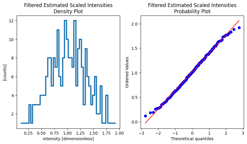
Estimated Scaled Intensities.#
[7]:
import scipy.stats as stats
import matplotlib.pyplot as plt

fig, (density_ax, prob_ax) = plt.subplots(1, 2, figsize=(10, 5))

densities = sc.values(results[FilteredEstimatedScaledIntensities].data).values
sc.values(results[FilteredEstimatedScaledIntensities].data).hist(intensity=50).plot(
    title="Filtered Estimated Scaled Intensities\nDensity Plot",
    grid=True,
    linewidth=3,
    ax=density_ax,
)
stats.probplot(densities, dist="norm", plot=prob_ax)
prob_ax.set_title("Filtered Estimated Scaled Intensities\nProbability Plot")
[7]:
Text(0.5, 1.0, 'Filtered Estimated Scaled Intensities\nProbability Plot')
Curve Fitting#
[8]:
import plopp as pp
import numpy as np
from ess.nmx.scaling import FittingResult

chebyshev_func = np.polynomial.chebyshev.Chebyshev(np.array([1, -1, 1]))
scale_function = np.vectorize(
    chebyshev_func / chebyshev_func(results[SelectedReferenceWavelength].value)
)
pp.plot(
    {
        "Original Data": results[FilteredEstimatedScaledIntensities],
        "Fit Result": results[FittingResult].fit_output,
    },
    grid=True,
    title="Fit Result [Intensities vs Wavelength]",
    marker={"Chebyshev": None, "Fit Result": None},
    linestyle={"Chebyshev": "solid", "Fit Result": "solid"},
)
[8]:

[9]:
reference_wavelength = sc.DataArray(
    data=sc.concat(
        [
            results[WavelengthScaleFactors].data.min(),
            results[WavelengthScaleFactors].data.max(),
        ],
        "wavelength",
    ),
    coords={
        "wavelength": sc.broadcast(
            results[SelectedReferenceWavelength], dims=["wavelength"], shape=[2]
        )
    },
)
wavelength_scale_factor_plot = pp.plot(
    {
        "scale_factor": results[WavelengthScaleFactors],
        "reference_wavelength": reference_wavelength,
    },
    title="Wavelength Scale Factors",
    grid=True,
    marker={"reference_wavelength": None},
    linestyle={"reference_wavelength": "solid"},
)
wavelength_scale_factor_plot.ax.set_xlim(2.8, 3.2)
reference_wavelength = results[SelectedReferenceWavelength].value
wavelength_scale_factor_plot.ax.text(
    3.0,
    0.25,
    f"{reference_wavelength=:} [{results[SelectedReferenceWavelength].unit}]",
    fontsize=8,
    color="black",
)
wavelength_scale_factor_plot
[9]:

Change Provider#
Here is an example of how to insert different filter function.
In this example, we will swap a provider that filters EstimatedScaledIntensities and provide FilteredEstimatedScaledIntensities.
After updating the providers, you can go back to Compute Desired Type and start over.
[10]:
from typing import NewType
import scipp as sc
from ess.nmx.scaling import (
    EstimatedScaledIntensities,
    FilteredEstimatedScaledIntensities,
)

# Define the new types for the filtering function
NRoot = NewType("NRoot", int)
"""The n-th root to be taken for the standard deviation."""
NRootStdDevCut = NewType("NRootStdDevCut", float)
"""The number of standard deviations to be cut from the n-th root data."""


def _calculate_sample_standard_deviation(var: sc.Variable) -> sc.Variable:
    """Calculate the sample variation of the data.

    This helper function is a temporary solution before
    we release new scipp version with the statistics helper.
    """
    import numpy as np

    return sc.scalar(np.nanstd(var.values))


# Define the filtering function with right argument types and return type
def cut_estimated_scaled_intensities_by_n_root_std_dev(
    scaled_intensities: EstimatedScaledIntensities,
    n_root: NRoot,
    n_root_std_dev_cut: NRootStdDevCut,
) -> FilteredEstimatedScaledIntensities:
    """Filter the mtz data array by the quad root of the sample standard deviation.

    Parameters
    ----------
    scaled_intensities:
        The scaled intensities to be filtered.

    n_root:
        The n-th root to be taken for the standard deviation.
        Higher n-th root means cutting is more effective on the right tail.
        More explanation can be found in the notes.

    n_root_std_dev_cut:
        The number of standard deviations to be cut from the n-th root data.

    Returns
    -------
    :
        The filtered scaled intensities.

    """
    # Check the range of the n-th root
    if n_root < 1:
        raise ValueError("The n-th root should be equal to or greater than 1.")

    copied = scaled_intensities.copy(deep=False)
    nth_root = copied.data ** (1 / n_root)
    # Calculate the mean
    nth_root_mean = nth_root.nanmean()
    # Calculate the sample standard deviation
    nth_root_std_dev = _calculate_sample_standard_deviation(nth_root)
    # Calculate the cut value
    half_window = n_root_std_dev_cut * nth_root_std_dev
    keep_range = (nth_root_mean - half_window, nth_root_mean + half_window)

    # Filter the data
    return FilteredEstimatedScaledIntensities(
        copied[(nth_root > keep_range[0]) & (nth_root < keep_range[1])]
    )


pl.insert(cut_estimated_scaled_intensities_by_n_root_std_dev)
pl[NRoot] = 4
pl[NRootStdDevCut] = 1.0

pl.compute(FilteredEstimatedScaledIntensities)
[10]:
scipp.DataArray (2.95 KB)
- wavelength: 180
- wavelength(wavelength)float32Å2.857202, 2.8588, ..., 3.1432657, 3.144864
Values:
array([2.857202 , 2.8588   , 2.8619962, 2.8635945, 2.8651924, 2.8667908,
       2.8683887, 2.869987 , 2.871585 , 2.8731833, 2.8747811, 2.8763795,
       2.8779774, 2.8795757, 2.8811736, 2.882772 , 2.8843699, 2.8859682,
       2.887566 , 2.8891644, 2.8907623, 2.8923607, 2.8939586, 2.895557 ,
       2.8971548, 2.8987532, 2.9003513, 2.9019494, 2.9035475, 2.9051456,
       2.906744 , 2.908342 , 2.9099402, 2.9115381, 2.9131365, 2.9147344,
       2.9163327, 2.9179306, 2.919529 , 2.9211268, 2.9227252, 2.924323 ,
       2.9259214, 2.9275193, 2.9291177, 2.9307156, 2.932314 , 2.9339118,
       2.9355102, 2.937108 , 2.9387064, 2.9403043, 2.9419026, 2.9435005,
       2.9450989, 2.9466968, 2.948295 , 2.949893 , 2.9514914, 2.9530892,
       2.9546876, 2.9562855, 2.9578838, 2.9594817, 2.96108  , 2.962678 ,
       2.9642763, 2.9658742, 2.9674726, 2.9690704, 2.9706688, 2.9722667,
       2.973865 , 2.975463 , 2.9770613, 2.9786592, 2.9802575, 2.9818554,
       2.9834538, 2.9850516, 2.98665  , 2.9882479, 2.9898462, 2.991444 ,
       2.9930425, 2.9946404, 2.9962387, 2.9978366, 2.999435 , 3.0010328,
       3.0026312, 3.004229 , 3.0058274, 3.0074253, 3.0090237, 3.0106215,
       3.01222  , 3.0138178, 3.0154161, 3.017014 , 3.0186124, 3.0202103,
       3.0218086, 3.0234065, 3.0250049, 3.0266027, 3.028201 , 3.029799 ,
       3.0313973, 3.0329952, 3.0345936, 3.0361915, 3.0377898, 3.0393877,
       3.040986 , 3.042584 , 3.0441823, 3.0457802, 3.0473785, 3.0489764,
       3.0505748, 3.0521727, 3.053771 , 3.055369 , 3.0569673, 3.0585651,
       3.0601635, 3.0617614, 3.0633597, 3.0649576, 3.066556 , 3.0681539,
       3.0697522, 3.07135  , 3.0729485, 3.0745463, 3.0761447, 3.0777426,
       3.079341 , 3.0809388, 3.0825372, 3.084135 , 3.0857334, 3.0873313,
       3.0889297, 3.0905275, 3.092126 , 3.0937238, 3.0953221, 3.0969203,
       3.0985184, 3.1001165, 3.1017146, 3.1033127, 3.1049109, 3.106509 ,
       3.108107 , 3.1097052, 3.1113033, 3.1129014, 3.1144996, 3.1160977,
       3.1176958, 3.119294 , 3.120892 , 3.1224904, 3.1240883, 3.1256866,
       3.1272845, 3.128883 , 3.1304808, 3.1320791, 3.133677 , 3.1352754,
       3.1368732, 3.1384716, 3.1400695, 3.1416678, 3.1432657, 3.144864 ],
      dtype=float32)
- (wavelength)float32𝟙0.6070114, 0.6354325, ..., 1.4262968, 1.4329288σ = 0.007581526, 0.009966516, ..., 0.015530329, 0.015853887
Values:
array([0.6070114 , 0.6354325 , 0.61014795, 0.6068784 , 0.6406334 ,
       0.64477855, 0.63060856, 0.63542855, 0.6324167 , 0.6801704 ,
       0.64791816, 0.652414  , 0.6717658 , 0.6621639 , 0.6798379 ,
       0.7657368 , 0.6897617 , 0.6949786 , 0.68923384, 0.6942186 ,
       0.71312326, 0.71762073, 0.719248  , 0.71350837, 0.7397376 ,
       0.7398708 , 0.7309188 , 0.7652437 , 0.7870944 , 0.7594039 ,
       0.7531101 , 0.75556797, 0.76490945, 0.8025271 , 0.7721254 ,
       0.78140897, 0.7865576 , 0.80898607, 0.7910712 , 0.80424136,
       0.81415737, 0.8031877 , 0.8225756 , 0.82421577, 0.8191481 ,
       0.83883417, 0.8289338 , 0.83124685, 0.83585805, 0.8385015 ,
       0.84103566, 0.8469526 , 0.8568808 , 0.8694568 , 0.85906804,
       0.9218925 , 0.8691482 , 0.910457  , 0.88111806, 0.9104874 ,
       0.9135022 , 0.92319083, 0.90916634, 0.9476996 , 0.9178994 ,
       0.9017219 , 0.91642   , 1.0024371 , 0.9270845 , 0.9234043 ,
       0.9451939 , 0.9580411 , 0.95741826, 0.94907516, 0.9626036 ,
       0.9487712 , 0.9515659 , 0.9979782 , 0.9831484 , 0.9640661 ,
       0.9879607 , 0.9713198 , 0.9780923 , 1.0047737 , 0.98358345,
       0.9882377 , 0.99075764, 1.018909  , 1.0000254 , 1.0028013 ,
       1.0172088 , 1.024566  , 1.0286235 , 1.0433916 , 1.1104821 ,
       1.0264289 , 1.0312595 , 1.0576755 , 1.0381942 , 1.0659459 ,
       1.0475025 , 1.0555083 , 1.0599737 , 1.0647993 , 1.1044763 ,
       1.0716054 , 1.085836  , 1.1003727 , 1.0791866 , 1.096032  ,
       1.0906415 , 1.1422418 , 1.1413152 , 1.1131383 , 1.1150991 ,
       1.1492105 , 1.1475223 , 1.1539438 , 1.1373259 , 1.12481   ,
       1.1319934 , 1.1355053 , 1.1449871 , 1.1513128 , 1.1601958 ,
       1.1492685 , 1.2059618 , 1.1931733 , 1.2093873 , 1.172439  ,
       1.1882433 , 1.2029705 , 1.2417048 , 1.1958982 , 1.192574  ,
       1.2114031 , 1.2002187 , 1.2199563 , 1.2094076 , 1.256482  ,
       1.2189393 , 1.2234412 , 1.2631079 , 1.2533275 , 1.246985  ,
       1.2448152 , 1.2749248 , 1.2598064 , 1.2584211 , 1.26102   ,
       1.2679971 , 1.2830582 , 1.2782192 , 1.2803183 , 1.2984796 ,
       1.2955241 , 1.308334  , 1.3730578 , 1.307733  , 1.3506969 ,
       1.316869  , 1.3708428 , 1.3499488 , 1.3652765 , 1.3402617 ,
       1.3605239 , 1.3775644 , 1.3633896 , 1.385249  , 1.3687915 ,
       1.381712  , 1.3882626 , 1.3878992 , 1.4007676 , 1.4101408 ,
       1.4342211 , 1.4354299 , 1.4360559 , 1.4262968 , 1.4329288 ],
      dtype=float32)

Variances (σ²):
array([5.74795376e-05, 9.93314388e-05, 3.98175434e-05, 5.14143139e-05,
       6.59856814e-05, 6.35042234e-05, 5.12313964e-05, 5.03618030e-05,
       5.48519383e-05, 6.64681502e-05, 5.44289178e-05, 5.28388628e-05,
       6.18483537e-05, 6.49031790e-05, 5.17519657e-05, 1.58387702e-04,
       5.97466023e-05, 6.94945847e-05, 6.17728219e-05, 6.55613185e-05,
       6.64384133e-05, 6.10811840e-05, 6.79638761e-05, 6.27376867e-05,
       6.04419656e-05, 5.94244702e-05, 6.86752101e-05, 6.63347600e-05,
       1.16998461e-04, 7.06466308e-05, 7.18489682e-05, 6.07973707e-05,
       6.64159816e-05, 9.21256287e-05, 7.51157058e-05, 7.64880751e-05,
       7.49804167e-05, 8.41489455e-05, 8.22133006e-05, 8.44401584e-05,
       8.60130967e-05, 8.42609152e-05, 9.90535991e-05, 8.61488079e-05,
       8.50271390e-05, 8.76785271e-05, 8.34146922e-05, 7.02328107e-05,
       1.00364952e-04, 9.05520501e-05, 9.42670522e-05, 9.19481608e-05,
       9.79183460e-05, 9.65009240e-05, 8.78656865e-05, 1.20414938e-04,
       9.97904062e-05, 1.23560938e-04, 9.40254249e-05, 1.04686864e-04,
       1.14489587e-04, 1.22188212e-04, 1.13109927e-04, 1.28414715e-04,
       1.25353123e-04, 1.21911195e-04, 9.33227857e-05, 1.74027431e-04,
       1.04913488e-04, 1.25347389e-04, 1.10791552e-04, 1.26701852e-04,
       1.09050285e-04, 1.24742073e-04, 1.30781860e-04, 1.05761384e-04,
       1.11854650e-04, 1.41779499e-04, 1.31608744e-04, 1.30743283e-04,
       1.20826429e-04, 1.26319152e-04, 1.34927235e-04, 1.38158532e-04,
       1.27356092e-04, 1.19864315e-04, 1.11187808e-04, 1.48789157e-04,
       1.01213933e-04, 1.20698089e-04, 1.43554687e-04, 1.38697913e-04,
       1.25700622e-04, 1.37931595e-04, 1.61406861e-04, 1.37677387e-04,
       1.58749288e-04, 1.38160191e-04, 1.55284506e-04, 1.42545759e-04,
       1.27560212e-04, 1.42550489e-04, 1.49925720e-04, 1.52065113e-04,
       1.55441434e-04, 1.23287304e-04, 1.55261441e-04, 1.44539532e-04,
       1.24982442e-04, 1.57909060e-04, 1.49287778e-04, 2.06205310e-04,
       1.90313207e-04, 1.77068432e-04, 1.71384701e-04, 1.79194976e-04,
       1.81565265e-04, 1.82234216e-04, 1.63582881e-04, 1.53892339e-04,
       1.61651551e-04, 1.55816175e-04, 1.77663547e-04, 1.43336118e-04,
       1.79886978e-04, 1.44532270e-04, 2.15440523e-04, 1.78006536e-04,
       1.68227794e-04, 1.43395737e-04, 1.68639366e-04, 2.08071913e-04,
       2.88074225e-04, 1.69707899e-04, 2.09134174e-04, 1.68616767e-04,
       1.68781975e-04, 1.89460785e-04, 1.70585758e-04, 2.13972060e-04,
       1.83197044e-04, 1.77821799e-04, 2.12173894e-04, 1.94450797e-04,
       2.00403243e-04, 2.15643304e-04, 1.80441697e-04, 2.11129067e-04,
       2.12913204e-04, 2.02940195e-04, 1.92602383e-04, 1.97268106e-04,
       2.11366874e-04, 2.23142299e-04, 2.23695009e-04, 1.99477669e-04,
       2.05906850e-04, 2.75295926e-04, 2.21289927e-04, 2.34401392e-04,
       2.12831786e-04, 2.33427883e-04, 2.35852815e-04, 2.32453123e-04,
       2.25265467e-04, 2.60025292e-04, 2.28782679e-04, 2.31453407e-04,
       2.34481500e-04, 2.85590824e-04, 3.04085901e-04, 2.48227967e-04,
       2.44201190e-04, 2.40701804e-04, 2.76635052e-04, 2.38082663e-04,
       2.61420006e-04, 2.59264576e-04, 2.41191126e-04, 2.51345773e-04],
      dtype=float32)