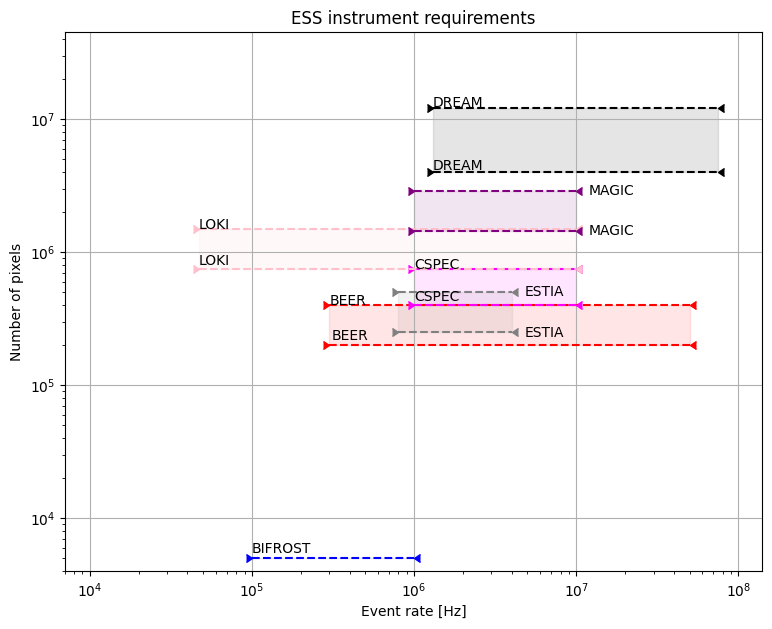
ESS Instruments

beamlime is designed and implemented to support live data reduction at ESS.

ESS has various instruments and each of them has different range of computation loads.

Here is the plot of number of pixel and event rate ranges.

from ess_requirements import ESSInstruments

ess_requirements = ESSInstruments()
ess_requirements.show()

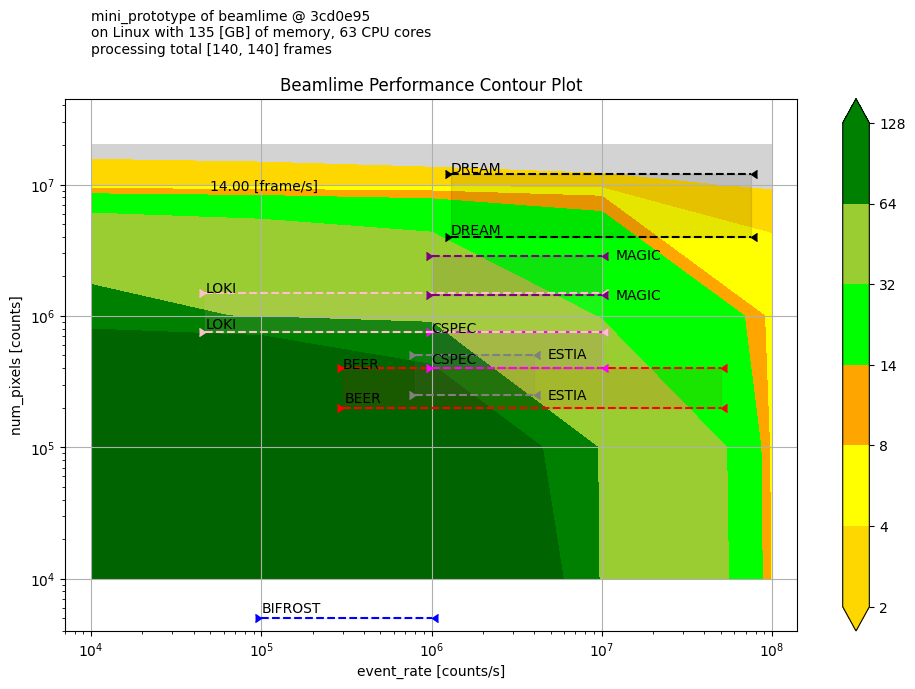
There is a set of benchmark results we have collected with dummy workflow in various computing environments.

They are collected with the benchmarks module in tests package in the repository.

And the benchmarks module also has loading/visualization helpers.

Here is a contour performance plot of one of the results.

from loader import collect_reports, merge_measurements
from docs.about.data import benchmark_results
import json

results = benchmark_results()
results_map = json.loads(results.read_text())
report_map = collect_reports(results_map)
df = merge_measurements(report_map)

Downloading file 'benchmark_results.json' from 'https://public.esss.dk/groups/scipp/beamlime/benchmarks/benchmark_results.json' to '/home/runner/.cache/beamlime/0'.

# Flatten required hardware specs into columns.
from environments import BenchmarkEnvironment


def retrieve_total_memory(env: BenchmarkEnvironment) -> float:
    return env.hardware_spec.total_memory.value


def retrieve_cpu_cores(env: BenchmarkEnvironment) -> float:
    return env.hardware_spec.cpu_spec.process_cpu_affinity.value


df["total_memory [GB]"] = df["environment"].apply(retrieve_total_memory)
df["cpu_cores"] = df["environment"].apply(retrieve_cpu_cores)

# Fix column names to have proper units.
df.rename(
    columns={
        "num_pixels": "num_pixels [counts]",
        "num_events": "num_events [counts]",
        "num_frames": "num_frames [counts]",
        "event_rate": "event_rate [counts/s]",
    },
    inplace=True,
)

import scipp as sc
from scipp.compat.pandas_compat import from_pandas, parse_bracket_header

# Convert to scipp dataset.
ds: sc.Dataset = from_pandas(
    df[df["target-name"] == "mini_prototype"].drop(columns=["environment"]),
    header_parser=parse_bracket_header,
    data_columns="time",
)

# Derive speed from time measurements and number of frames.
ds["speed"] = ds.coords["num_frames"] / ds["time"]

from calculations import sample_mean_per_bin, sample_variance_per_bin

# Calculate mean and variance per bin.
binned = ds["speed"].group("event_rate", "num_pixels", "cpu_cores")
da = sample_mean_per_bin(binned)
da.variances = sample_variance_per_bin(binned).values

# Select measurement with 63 CPU cores.
da_63_cores = da["cpu_cores", sc.scalar(63, unit=None)]

# Create a meta string with the selected data.
df_63_cores = df[df["cpu_cores"] == 63].reset_index(drop=True)
df_63_cores_envs: BenchmarkEnvironment = df_63_cores["environment"][0]
meta_64_cores = [
    f"{ds.coords['target-name'][0].value} "
    f"of beamlime @ {df_63_cores_envs.git_commit_id[:7]} ",
    f"on {df_63_cores_envs.hardware_spec.operating_system} "
    f"with {df_63_cores_envs.hardware_spec.total_memory.value} "
    f"[{df_63_cores_envs.hardware_spec.total_memory.unit}] of memory, "
    f"{da_63_cores.coords['cpu_cores'].value} CPU cores",
    f"processing total [{df_63_cores['num_frames [counts]'].min()}, {df_63_cores['num_frames [counts]'].max()}] frames ",
]

# Draw a contour plot.
from matplotlib import pyplot as plt
from visualize import plot_contourf

fig, ax = plt.subplots(1, 1, figsize=(10, 7))
ctr = plot_contourf(
    da_63_cores,
    x_coord="event_rate",
    y_coord="num_pixels",
    fig=fig,
    ax=ax,
    levels=[2, 4, 8, 14, 32, 64, 128],
    extend="both",
    colors=["gold", "yellow", "orange", "lime", "yellowgreen", "green", "darkgreen"],
    under_color="lightgrey",
    over_color="darkgreen",
)
ess_requirements.plot_boundaries(ax)
ess_requirements.configure_full_scale(ax)

ax.set_title("Beamlime Performance Contour Plot")
ax.annotate("14.00 [frame/s]", (5e4, 9e6), size=10)
ax.text(10**4, 10**8, "\n".join(meta_64_cores))
fig.tight_layout()

Performance Comparisons

We will compare performances of different memory capacity and number of cpu cores.

Performance differences are calculated with the following function difference.

def difference(da: sc.DataArray, standard_da: sc.DataArray) -> sc.DataArray:
    """Difference from the standard data array in percent."""

    return sc.scalar(100, unit="%") * (da - standard_da) / standard_da

Memory

More memory capacity did not make any meaningful performance improvement tendency.

memory_comparison_line_plot

CPU Cores

More CPU cores showed improved performance for most cases, especially bigger number of events.

It was expected due to multi-threaded computing of scipp.

cpu_comparison_line_plot